
Backtesting a Dynamic Investment Strategy with Python
8 minute read
← Previous Post AI Trading Strategies Intro
In this blog, I focus on financial data analysis specifically evaluating returns and backtesting. This study was inspired from concepts and exercises practiced in Udacity’s AI Trading Strategies Nanodegree Course 4. In this project, using Python-based workflows, I explored how to prepare financial data for quantitative analysis and evaluate the risk adjusted returns of a dynamic risk parity weighted investment strategy .
Project Objectives
The purpose of this project is to develop a working template for evaluating dynamic investment strategies. The primary goals are:
- Collect asset and risk-free rate data using Python.
- Generate and compare Fixed Weight and Risk Parity portfolio strategies.
- Measure and visualize risk and return metrics using industry-standard performance indicators.
- Practice a workflow that can be extended to personal and professional investment research.
Data Collection
To have a well-diversified portfolio, I selected three representative assets from different classes:
- AGG: Bonds (iShares Core U.S. Aggregate Bond ETF)
- GLD: Gold (SPDR Gold Shares)
- QQQ: Equities (Invesco QQQ Trust)
All data was collected using the yfinance Python package at daily frequency, then resampled to monthly for consistency in evaluation.
Additionally, I pulled the 13-week Treasury Bill rate using the ticker ^IRX as a risk-free rate proxy. This rate was used to compute excess returns and adjust various risk metrics.
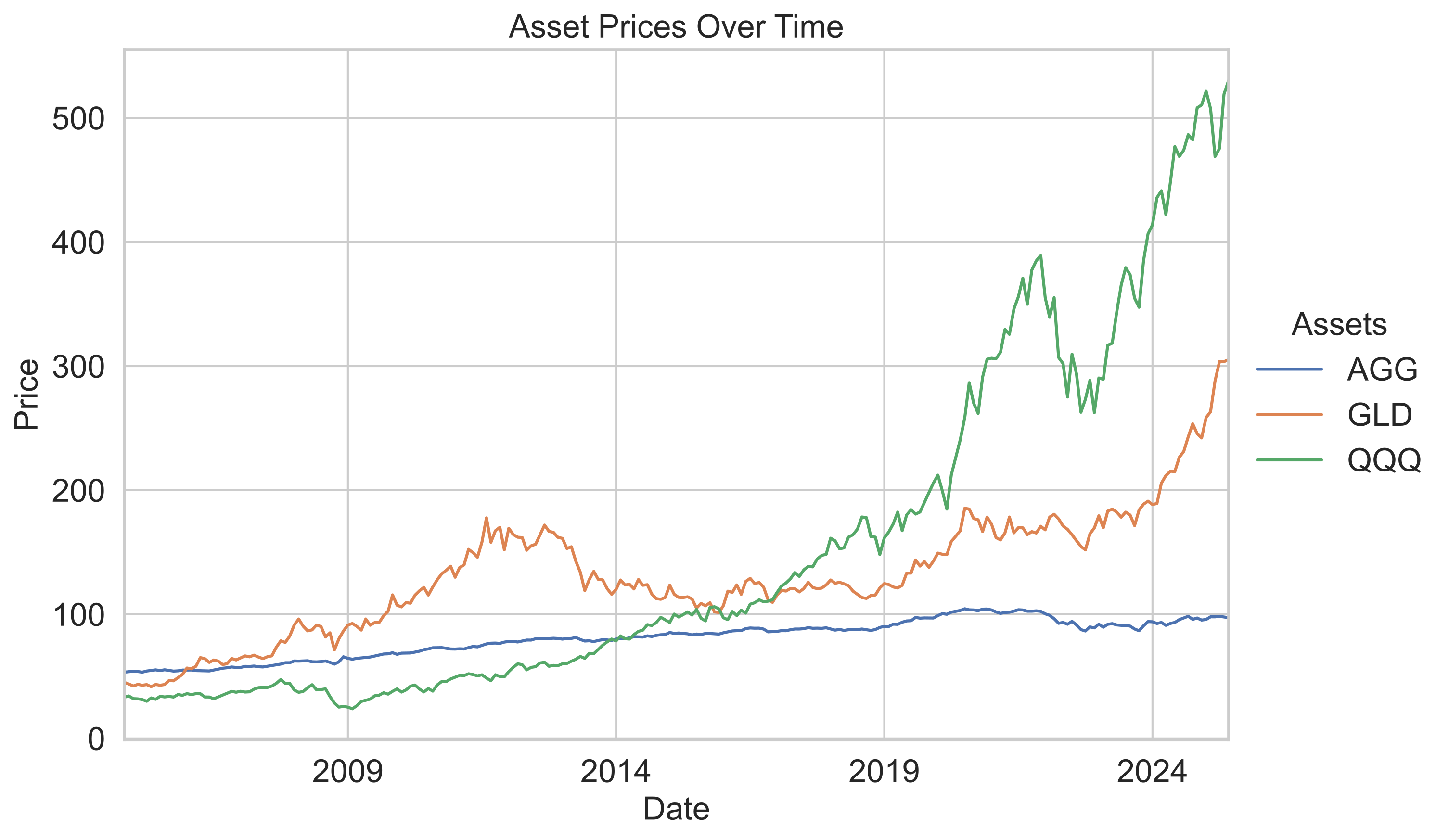
Monthly variation in asset prices over the backtest period.
- AGG (Bonds):
- Delivered steady and low-volatility growth throughout the period.
- Served as a stable anchor for the portfolio with minimal drawdowns.
- GLD (Gold):
- Strong gains from 2007 to 2012, then mostly flat, with another surge after 2019.
- Acted as a hedge during market stress and inflationary periods, but experienced long periods of sideways movement.
- QQQ (Tech Stocks):
- Modest growth until 2012, followed by explosive gains, especially post-2019.
- Highest volatility and the primary driver of overall portfolio growth, but with occasional sharp corrections.
Overall
- The combination of AGG, GLD, and QQQ provided diversification: AGG stabilized returns, GLD offered crisis protection, and QQQ delivered strong long-term growth.
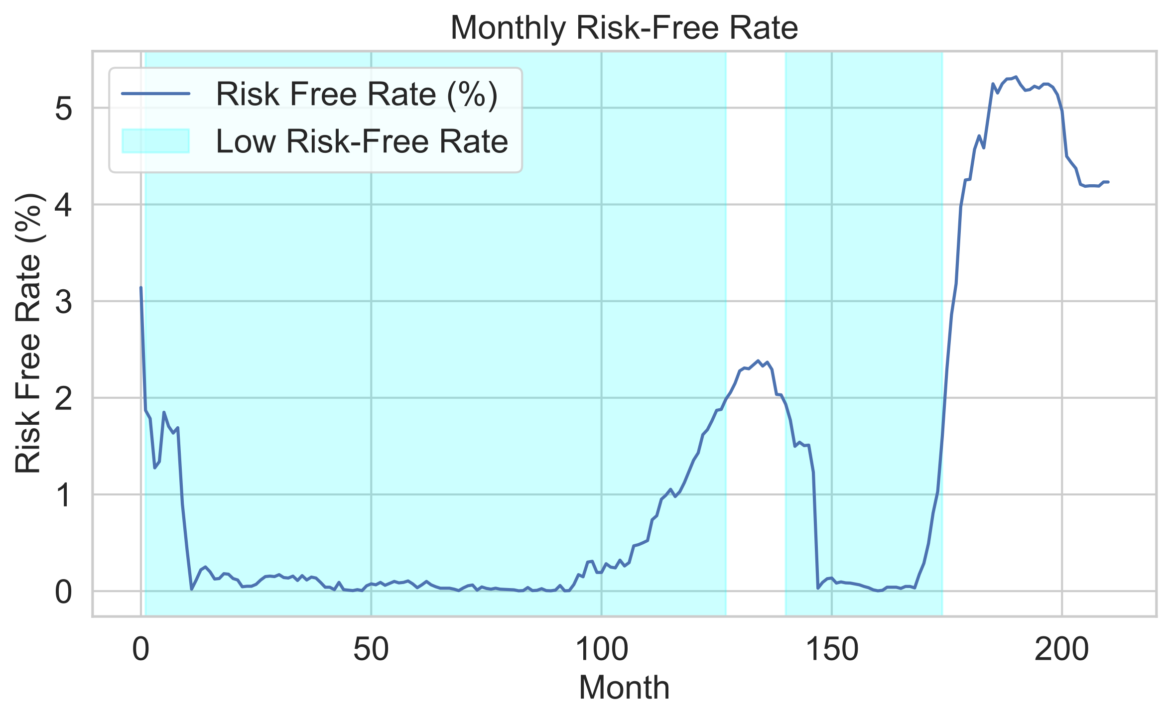
Risk-free rate resampled from daily data by taking the last value of each month.
- 2008–2015:
- Risk-free rate dropped sharply and stayed near historic lows.
- Cause: Global Financial Crisis and subsequent quantitative easing by central banks.
- 2016–2019:
- Gradual increase in the risk-free rate as economic recovery gained momentum.
- Cause: Federal Reserve rate hikes during the post-crisis recovery phase.
- 2020:
- Sharp decline back to near-zero levels.
- Cause: COVID-19 pandemic triggered emergency rate cuts to stimulate the economy.
- 2022–2024:
- Steep rise in the risk-free rate to levels not seen since before 2008.
- Cause: Aggressive Federal Reserve rate hikes to combat high inflation post-pandemic.
Key Takeaway
- The risk-free rate has seen three distinct regimes: prolonged lows after 2008, a moderate rise pre-pandemic, a crash in 2020, and a rapid surge from 2022 onward due to inflationary pressures and tightening monetary policy.
Data Transformation
Once collected, the data underwent several transformations:
- Monthly Returns: Log returns were computed from resampled monthly closing prices.
- Resampled Risk-Free Rate: The daily risk-free yield was annualized and converted into equivalent monthly return.
- Return Adjustment: Excess returns were computed by subtracting the monthly risk-free rate from asset returns.
These monthly returns formed the basis for all further evaluation and backtesting procedures.
Volatility Estimation and Risk Parity Weights
For the Risk Parity strategy, the weight allocation was dynamically adjusted using rolling volatility:
- A 36-month rolling window was used to estimate standard deviation for each asset.
- Risk Parity weights were computed by assigning weight inversely proportional to volatility.
- The weights were normalized to sum to one for each month.
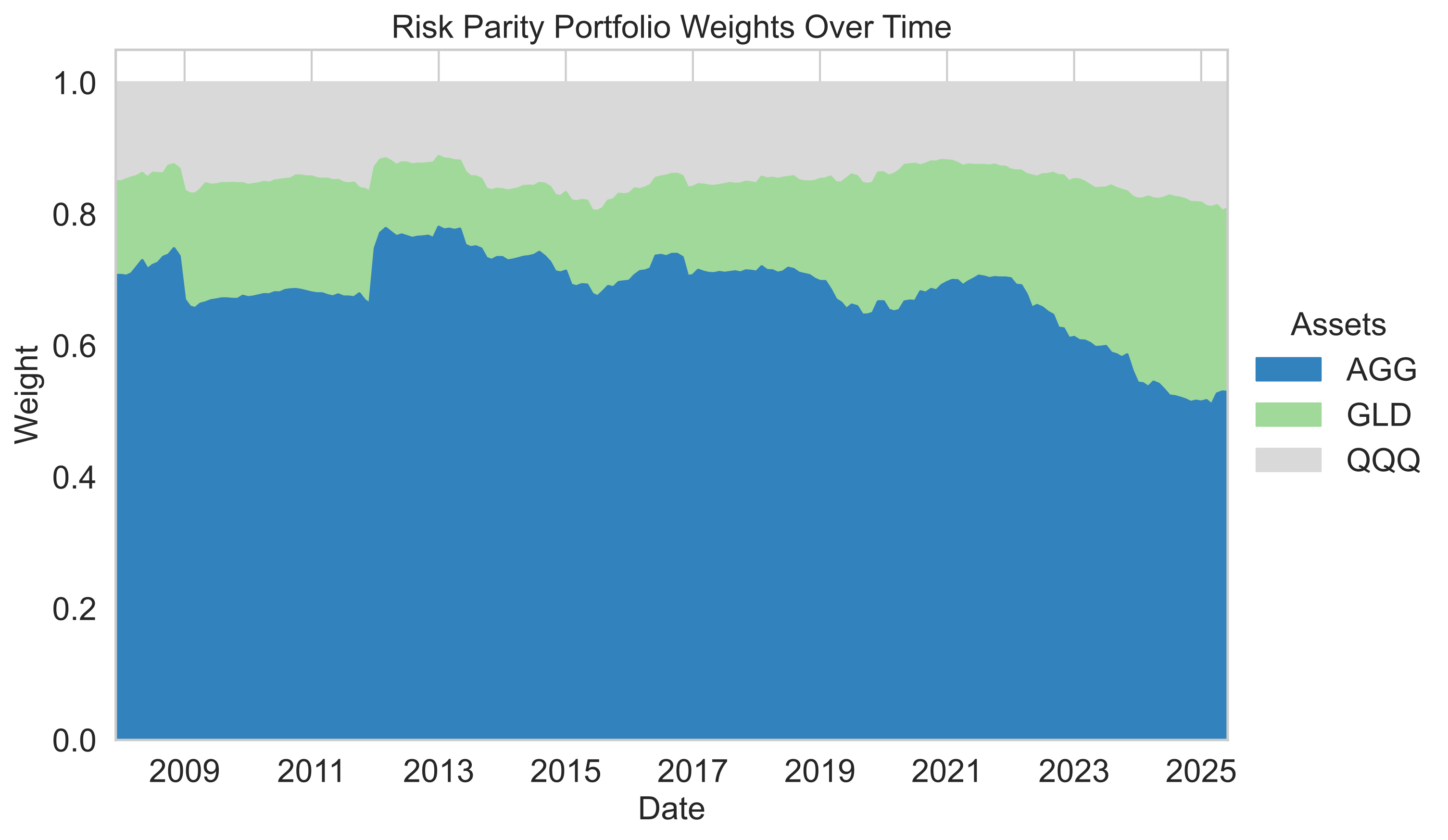
Risk Parity assigns higher weights to less volatile assets dynamically over time.
- AGG (Bonds):
- Consistently received the highest weight in the risk parity allocation.
- Weight has declined in recent periods but remained dominant overall.
- GLD (Gold):
- Started with a low allocation, but weight increased over time.
- Shows periods of upward trend, especially in recent years.
- QQQ (Tech Stocks):
- Maintained the lowest allocation throughout most of the period.
- Weight increased slightly in later years, but still lagged behind AGG and GLD.
Key Takeaway
- Risk parity allocation favored AGG due to its low volatility, while GLD’s share grew as its risk profile changed. QQQ remained the smallest component because of its higher risk, despite its strong returns.
Portfolio Return and Performance Evaluation
Using the calculated weights (both static and dynamic), portfolio returns were generated and evaluated using the following metrics:
| Metric | Description |
|---|---|
| Annualized Return | Average yearly return |
| Annualized Volatility | Standard deviation of yearly returns |
| Downside Volatility | Volatility considering only negative returns |
| Max Drawdown | Largest drop from peak to trough |
| Sharpe Ratio | Return relative to total risk |
| Sortino Ratio | Return relative to downside risk |
| Calmar Ratio | Return relative to max drawdown |
| Value-at-Risk (VaR) | Estimated worst-case monthly loss |
| Conditional VaR (CVaR) | Average loss beyond the VaR threshold |
| Skewness and Kurtosis | Measures asymmetry and tail risk |
| Excess Return | Return above the risk-free benchmark |
Visual tools like equity curves and drawdown charts were also used to provide better interpretation of strategy stability.
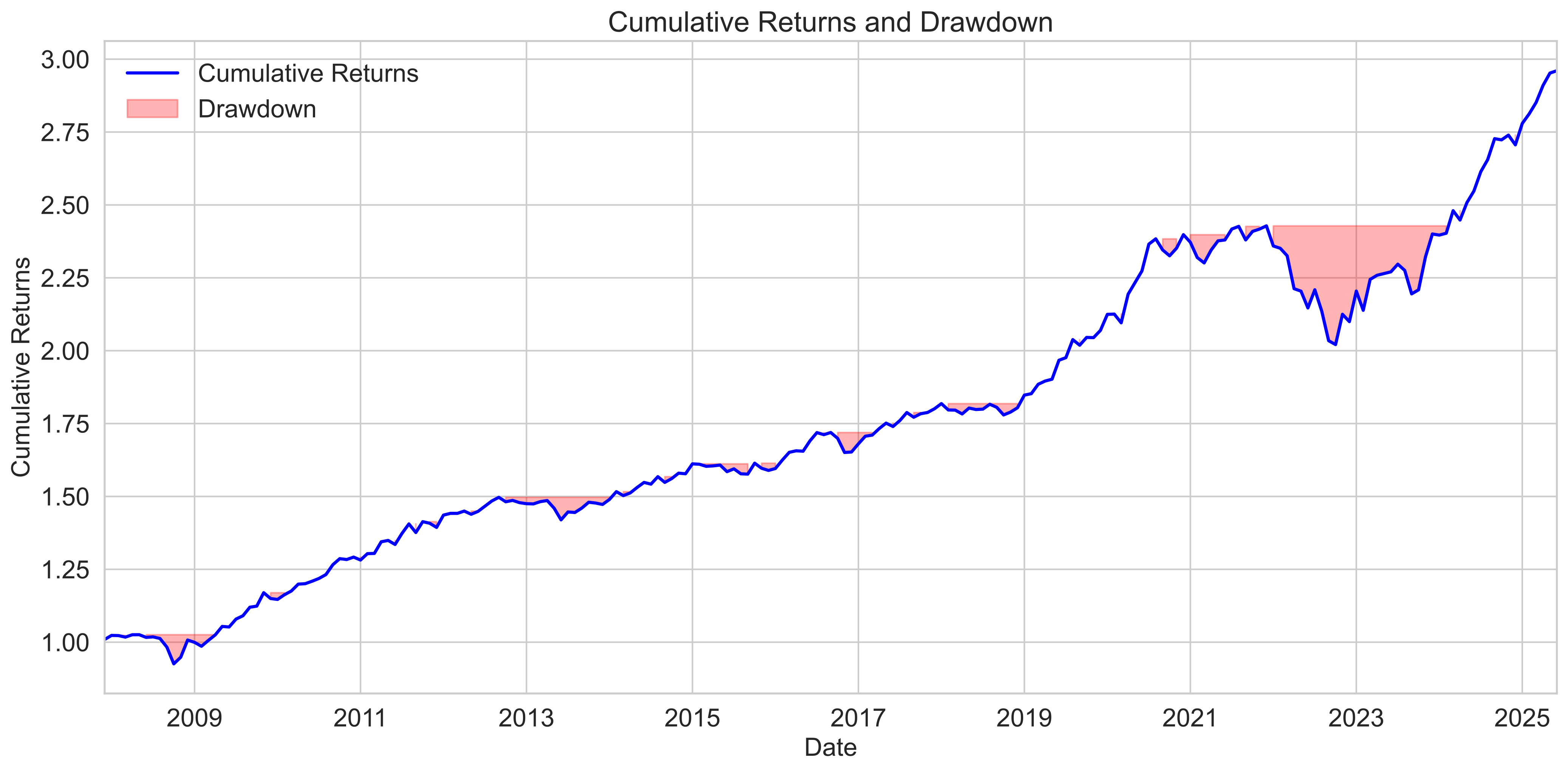
Drawdowns highlight capital declines from peak, useful to understand downside exposure.
- Cumulative Returns:
- The portfolio shows a steady upward trend in cumulative returns over time.
- Growth is largely uninterrupted, especially in the second half of the period, indicating robust long-term performance.
- Drawdown:
- Drawdowns (highlighted in red) are generally shallow and short-lived for most of the period.
- A notable period of deeper and more prolonged drawdowns occurs in the later stage, but the portfolio recovers quickly to new highs.
Key Takeaway
- The portfolio demonstrates strong compounding and resilience, with limited and recoverable drawdowns.
- This reflects effective risk management and the ability to weather market downturns without significant or sustained losses.
Fixed Weight vs Risk Parity Comparison
The core of this project was to compare the static Fixed Weight portfolio versus the dynamic Risk Parity portfolio.
| Metric | Risk Parity | Fixed Weight |
|---|---|---|
| Ann. Return | 6.37% | 6.71% |
| Ann. Volatility | 6.11% | 6.86% |
| Max Drawdown | 16.8% | 17.3% |
| Sharpe Ratio | 0.85 | 0.80 |
| Sortino Ratio | 1.24 | 1.17 |
| Calmar Ratio | 0.38 | 0.39 |
| VaR | 2.41% | 2.70% |
| CVaR | 3.57% | 4.04% |
| Excess Return | 5.16% | 5.50% |
A clear trade-off: Fixed Weight offers slightly higher returns but also higher volatility and tail risk.
- Fixed Weight (orange) generally achieves higher mean return and higher volatility compared to Risk Parity (green).
- Risk Parity consistently demonstrates lower downside volatility, max drawdown, VaR, and CVaR, indicating better downside and tail risk control.
- Sharpe and Sortino ratios are higher for Risk Parity, highlighting its superior risk-adjusted performance.
- Fixed Weight shows slightly higher Calmar ratio and excess return, reflecting its stronger overall growth despite higher drawdowns.
- Both strategies exhibit similar kurtosis, but Fixed Weight is more negatively skewed, suggesting greater exposure to negative outlier events.
Key Takeaway:
- Risk Parity excels in risk management and risk-adjusted returns.
- Fixed Weight delivers greater total returns, accepting more risk and larger drawdowns in the process.
Insights and Takeaways
This project went beyond just following instructions. By integrating outside material and additional benchmarks, I gained a more nuanced understanding of portfolio strategy design.
- Adding VaR and CVaR from outside reading helped me understand worst-case and tail risks in ways that Sharpe or Sortino cannot capture.
- Creating a Fixed Weight benchmark gave clarity: Risk Parity isn’t just about smoothing volatility — it’s about disciplined adaptation to changing market conditions.
- I particularly enjoyed implementing Risk Parity weights using rolling volatility and tracking how dynamic weight adjustments changed portfolio behavior.
- Throughout the notebook, I actively pursued modular and reusable code design. Each major step in the workflow was encapsulated into clearly defined Python functions. This not only improved code readability but also made the analysis easier for comparison of the considered strategies as well as potential future experimentation. This modular approach will make it easier to expand the notebook into a full backtesting framework for other strategies such as Kelly rotation or SPX 0DTE spread logic.
- This exercise provides a solid foundation for constructing rule-based strategies that adapt to market conditions.
These insights made the project much more engaging and helped connect theoretical learning to real-world strategy development.
Stay tuned as I progress through the remaining Nanodegree course projects and beyond, each accompanied by detailed blog breakdowns:
- Building a Reinforcement Learning Trading Model
- Building and Optimizing a Classification Model for Trading
- Building a Momentum-Based Algorithmic Trading Program
Thanks for reading!
← Previous Post AI Trading Strategies Intro