Wi-Fi Fingerprint Indoor Localization (Part II): Latitude-Longitude Regression

September 03, 2017 19 minute read

This post is part of a series of blogs on machine learning approaches for Wi-Fi fingerprinting based indoor localization.

In the previous post, we performed various transformations on the independent variables of the raw UJIIndoorLoc dataset to prepare it for the machine learning.

In this notebook, first, I focus on our response variables including building ID, floor ID, latitiude and longitude. Understanding the class imbalance in classification responses buildingID and floorID is important for training our machine learning models. Similarly, I analyze the distributions of our regression response variables latitude and longitude and their relationship with the building ID and floor ID. Second, I formulate the localization problem for the machine learning. Finally, I begin constructing machine learning framework first by focusing on regression without Floor and Building information. In future notebooks, I will model and evaluate cascade machine learning frameworks that perform building and floor classification before applying building and floor-optimized regression models.

1. Setup

# Data Collection and Transformations
import numpy as np
import pandas as pd
import datetime as dt
import time
import pickle
from sklearn.preprocessing import Imputer, StandardScaler
from itertools import cycle

# Statistical Testing
import statsmodels.api as sm
from statsmodels.formula.api import ols
import scipy

# Machine Learning
from sklearn.model_selection import train_test_split, cross_val_score
from sklearn.preprocessing import PolynomialFeatures
from sklearn.decomposition import PCA
from sklearn.model_selection import learning_curve, validation_curve
from sklearn.model_selection import GridSearchCV
from sklearn.pipeline import Pipeline

# Regression
from sklearn.linear_model import LinearRegression, Lasso, Ridge
from sklearn.kernel_ridge import KernelRidge
from sklearn.neighbors import KNeighborsRegressor, KNeighborsClassifier
from sklearn.tree import ExtraTreeRegressor
from sklearn.ensemble import RandomForestRegressor, ExtraTreesRegressor
from sklearn.multioutput import MultiOutputRegressor
from sklearn.svm import SVR
from sklearn.neural_network import MLPRegressor
import xgboost as xgb
from xgboost.sklearn import XGBRegressor

# Class imbalance
from imblearn.over_sampling import SMOTE
from imblearn.under_sampling import NearMiss
from imblearn.pipeline import make_pipeline

# Classification
from sklearn.linear_model import LogisticRegression
from sklearn.naive_bayes import GaussianNB
from sklearn.ensemble import RandomForestClassifier, ExtraTreesClassifier, AdaBoostClassifier
from sklearn.svm import SVC
from sklearn.metrics import roc_curve, auc, classification_report, accuracy_score
from sklearn.preprocessing import label_binarize
from sklearn.multiclass import OneVsRestClassifier
from scipy import interp

# Plotting
from mlxtend.plotting import plot_learning_curves
import matplotlib
import matplotlib.pyplot as plt
from matplotlib.colors import ListedColormap
plt.rcParams['figure.figsize'] = [10,8]
import seaborn as sns
%matplotlib inline

import warnings
warnings.filterwarnings('ignore')

Loading the transformed data from our previous notebook.

X_pca_crossval = pd.read_csv("data/X_pca_crossval.csv",index_col=0)
y_crossval = pd.read_csv("data/y_crossval.csv",index_col=0)

X_pca_holdout = pd.read_csv("data/X_pca_holdout.csv",index_col=0)
y_holdout = pd.read_csv("data/y_holdout.csv",index_col=0)

X_raw_crossval = pd.read_csv("data/X_raw_crossval.csv",index_col=0)
X_raw_holdout = pd.read_csv("data/X_raw_holdout.csv",index_col=0)

X_pca_crossval.shape,y_crossval.shape,X_pca_holdout.shape,y_holdout.shape

((17874, 150), (17874, 6), (1987, 150), (1987, 6))

X_raw_crossval.fillna(value=100,inplace=True)
X_raw_holdout.fillna(value=100,inplace=True)

y_crossval.head()

	LONGITUDE	LATITUDE	FLOOR	BUILDINGID	SPACEID	RELATIVEPOSITION
14651	-7367.4588	4.864842e+06	1	2	117	2
16771	-7594.2641	4.864982e+06	3	0	108	2
17601	-7596.2032	4.864982e+06	3	0	107	2
6651	-7322.5876	4.864821e+06	0	2	103	2
86	-7384.2113	4.864776e+06	3	2	222	2

In the next few sections, we explore the characteristics of the different response variables.

2. Response EDA

2.1 Building EDA

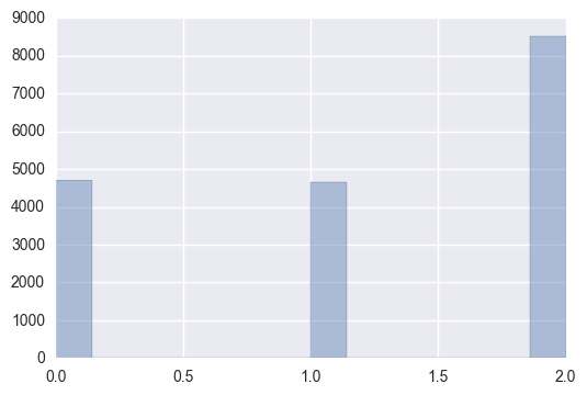
sns.distplot(y_crossval[['BUILDINGID']],kde=False)

<matplotlib.axes._subplots.AxesSubplot at 0x108053d68>

png

Observations:

In our training samples, building 2 has the clear majority with it’s count being slightly lower than the sum of building 0 and building 1.
Building 0 and building 1 have roughly the same representation in the training data.

Clearly, there is an imbalance among the groups.

markers = ('s', 'x', 'o', '^', 'v')
colors = ('red', 'blue', 'lightgreen', 'gray', 'cyan')
cmap = ListedColormap(colors[:len(np.unique(y_crossval['BUILDINGID']))])

for idx, cl in enumerate(np.unique(y_crossval['BUILDINGID'])):
        plt.scatter(x=y_crossval.loc[y_crossval.BUILDINGID== cl]['LATITUDE'],
                    y=y_crossval.loc[y_crossval.BUILDINGID== cl]['LONGITUDE'],
                    alpha=0.6,
                    c=cmap(idx),
                    edgecolor='black',
                    marker=markers[idx],
                    label=cl)

plt.xlabel('Latitude')
plt.ylabel('Longitude')
plt.legend(loc='upper right')
plt.tight_layout()

png

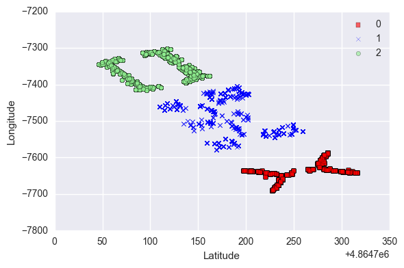
The above plot illustrates the locations of the buildings in the campus.

markers = ('s', 'x', 'o', '^', 'v')
colors = ('red', 'blue', 'lightgreen', 'gray', 'cyan')
cmap = ListedColormap(colors[:len(np.unique(y_crossval['BUILDINGID']))])

for idx, cl in enumerate(np.unique(y_crossval['BUILDINGID'])):
        plt.scatter(x=X_pca_crossval.loc[y_crossval.BUILDINGID== cl].iloc[:,0],
                    y=X_pca_crossval.loc[y_crossval.BUILDINGID== cl].iloc[:,1],
                    alpha=0.6,
                    c=cmap(idx),
                    edgecolor='black',
                    marker=markers[idx],
                    label=cl)

plt.xlabel('PCA Component 1')
plt.ylabel('PCA Component 2')
plt.legend(loc='lower right')
plt.tight_layout()

png

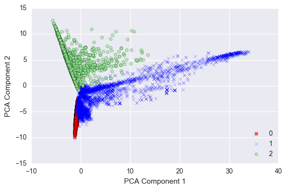
The above plot illustrates how the buildingID are distributed across the top two PCA dimensions. Later, I explore the machine learning approaches for the building classification.

Remember PCA is an unsupervised learning technique for dimensionality reduction. So, it is quite possible the two top PCA components might not have explained our response variable well.

2.2 Floor EDA

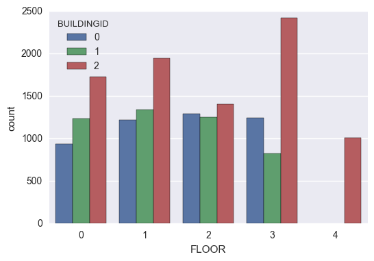
sns.countplot(x="FLOOR", hue="BUILDINGID", data=y_crossval,orient="v")

<matplotlib.axes._subplots.AxesSubplot at 0x10e135ac8>

png

Observations:

Buildings 0 and 1 have 4 floors whereas Building 2 has 5 floors.
Expectedly, the samples from Building 2 are consistently the highest across all the floors.

3. Problem Formulation

3.1 Error Metric

The overall goal of this project is to build models for accurate indoor localization. The mean positioning error expressed as the mean Euclidean distance between the real and estimated locations. However, in multi-building, multi-floor environments as in our problem, just the positioning error due to Euclidean distance is not enough. Wrong floor and wrong building classification are not desirable as the actual movement from the predicted location to the actual location might involve great displacement.

Therefore, we include penalty terms to the mean error equation to penalize failures in floor and building classification. This was introduced in the 2015 EvAAL-ETRI competition. The cost function can be expressed as follows:

$positioning_error(actual,predicted)= euclidean_distance(actual,predicted) + penalty_{floor}fail_{floor} + penalty_{building}fail_{building}$

where $fail_{floor}$ and $fail_{building}$ indicate if the floor and building are incorrectly identified, $penalty_{floor}$ and $penalty_{building}$ are the penalty values applied for wrongful classification of floor and building respectively. The penalty values were set to 4 and 50 respectively in the third track of the competition (Source). Expectedly, the penalty for building classification failure is higher than that of floor classification failure. In this project, I utilize the same penalty term values for the error metric.

3.2 Machine Learning Methodology

Because of the added penalty terms, we cannot simply perform regression for the Latitude and Longitude. Separate models might have to be trained per-floor and per-building. Hence, the building and floor need to be classified first.

However, I first analyze the regression variables in isolation without incorporating the buildingID and FloorID. The framework built will be used for comparison against the Cascade framework that incorporates the building and floor information.

4. Multi-Variable Multivariate Regression

The key concepts of building the regression framework include:

MultiOutputRegressor: We have the response as a vector of 2-dimensions (Latitude and Longitude). Not every regression method in scikit-learn can handle this sort of problem. Most linear models provide this capability but for those that don’t, a new class MultiOutputRegressor is available for parallelization of regressors for multivariate output.
Linear Regression Models: First, I will focus on Linear regression and its variants including Lasso, Kernel Ridge.
Polynomial Features: Consider Polynomial Features including quadratic and cubic for addressing non-linearities.
Other Regression Models: ExtraTreesRegressor, RandomForestRegressor, XGBoostRegressor
Stacking: Simple Average, XGBoost stacking as shown in this Kaggle kernel.

X_train = np.array(X_pca_crossval)
y_train = y_crossval[['LATITUDE','LONGITUDE']]

X_test = np.array(X_pca_holdout)
y_test = y_holdout[['LATITUDE','LONGITUDE']]

X_train.shape,y_train.shape,X_test.shape,y_test.shape

((17874, 150), (17874, 2), (1987, 150), (1987, 2))

# Dictionary to store nested cross-validation scores
model_scores = {}

# Dictionary to store model and param grid mapping
model_param_grid = {}

In the next few sub-sections, we perform nested cross-validation on the different model families. In nested cross-validation, the inner fold performs the parameter tuning and the outer fold is used for the validation performance.

Before we begin the model assessment, let’s write a function to simplify the nested cross-validation operation.

4.1 Nested Cross-Validation

def nested_crossval(reg_list,reg_labels, model_param_grid=model_param_grid, model_scores = model_scores,
                    X = X_train, y= y_train, label_extension = None):
    '''
    Inputs:
    reg_model        : List of Regression model instances
    reg_label        : List of Regression model labels
    model_param_grid : List of parameter grids
    X                : explanatory variables
    y                : response variable array
    model_scores     : Dictionary to store nested cross-validation scores
    label_extension  : Extension to regression label in model_scores key

    Outputs:
    model_scores     : Updated dictionary of nested cross-validation scores
    '''


    for reg_model, reg_label in zip(reg_list, reg_labels):

        #print(param_grid)

        gs = (GridSearchCV(estimator=reg_model,
                            param_grid=model_param_grid[reg_label],
                            cv=2,
                            scoring = 'neg_mean_squared_error',
                            n_jobs = 1))

        scores = cross_val_score(estimator=gs,
                                 X=X,
                                 y=y,
                                 cv=5,
                                 scoring='neg_mean_squared_error')
        scores = np.sqrt(np.abs(scores))

        if label_extension:
            reg_label += '_' + label_extension

        print("RMSE: %0.2f (+/- %0.2f) [%s]"
              % (scores.mean(), scores.std(), reg_label))

        model_scores[reg_label] = scores


    return model_scores

4.2 Linear Models and Variants

In this sub-section, I analyze the performance of Linear Regression models and its regularization variants.

## Linear Models

# Ridge Regression
pipe_ridge = Pipeline([('scl', StandardScaler()),
            ('reg', Ridge(random_state=1))])

# Lasso
pipe_lasso = Pipeline([('scl', StandardScaler()),
            ('reg', Lasso(random_state=1))])

param_grid_lm= {
    'reg__alpha':[0.01,0.1,1,10],
}

reg_lm = [pipe_ridge,pipe_lasso]
reg_labels_lm = ['Ridge','Lasso']
model_param_grid['Ridge'] = param_grid_lm
model_param_grid['Lasso'] = param_grid_lm

model_scores = nested_crossval(reg_lm,reg_labels_lm)

RMSE: 25.25 (+/- 0.41) [Ridge]
RMSE: 25.26 (+/- 0.43) [Lasso]

model_scores

{'Lasso': array([ 25.49069375,  24.50169635,  25.78675344,  25.24330896,  25.29979238]),
 'Ridge': array([ 25.43926941,  24.53596898,  25.780613  ,  25.20794527,  25.30487622])}

Interestingly, ridge regression and Lasso provide nearly the same performance but still very far from our baseline of 7.5m.

4.2 Polynomial Regression

In this sub-section, we analyze the non-linear variations of Regression by incorporating higher-order features into the Regression Analysis.

quadratic = PolynomialFeatures(degree=2)
X_quad = quadratic.fit_transform(X_train)

pipe_ridge_poly = Pipeline([('scl', StandardScaler()),
                            ('pca', PCA(n_components=100)),
                            ('reg', Ridge(random_state=1))])

# Lasso
pipe_lasso_poly = Pipeline([('scl', StandardScaler()),
                            ('pca', PCA(n_components=100)),
                            ('reg', Lasso(random_state=1))])

reg_lm_quad = [pipe_ridge_poly,pipe_lasso_poly]
reg_labels_lm_quad = ['Ridge_Quadratic','Lasso_Quadratic']
model_param_grid['Ridge_Quadratic'] = param_grid_lm
model_param_grid['Lasso_Quadratic'] = param_grid_lm

model_scores = nested_crossval(reg_lm_quad,reg_labels_lm_quad, X= X_quad)

# First, let's save our data into a file
f = open("model_scores_lm.pckl", "wb")
pickle.dump(model_scores,f)

pkl_file = open('model_scores_lm.pckl', 'rb')

model_scores = pickle.load(pkl_file)

cubic = PolynomialFeatures(degree=3)
X_cubic = cubic.fit_transform(X_train)

reg_lm_cube = [pipe_ridge_poly,pipe_lasso_poly]
reg_labels_lm_cube = ['Ridge_Cubic','Lasso_Cubic']
model_param_grid['Ridge_Cubic'] = param_grid_lm
model_param_grid['Lasso_Cubic'] = param_grid_lm

model_scores = nested_crossval(reg_lm_cube,reg_labels_lm_cube, X= X_cubic)

4.3 K Nearest Neighbors Regression

pipe_knn = Pipeline([('scl', StandardScaler()),
            ('reg', KNeighborsRegressor())])

grid_param_knn = {
    'reg__n_neighbors': [2,3,5,7],
    'reg__weights': ['uniform','distance'],
    'reg__metric': ['euclidean','minkowski','manhattan'],
    'reg__n_jobs': [-1]
}

model_param_grid['KNN'] = grid_param_knn

model_scores = nested_crossval([pipe_knn],['KNN'])

RMSE: 5.93 (+/- 0.26) [KNN]

# First, let's save our data into a file
f = open("model_scores_knn.pckl", "wb")
pickle.dump(model_scores,f)

model_scores

{'KNN': array([ 6.44366044,  5.9055819 ,  5.74672049,  5.7716296 ,  5.76268187]),
 'Lasso': array([ 25.49069375,  24.50169635,  25.78675344,  25.24330896,  25.29979238]),
 'Ridge': array([ 25.43926941,  24.53596898,  25.780613  ,  25.20794527,  25.30487622])}

4.4 Tree-Based Models

# Random Forests
reg_rf = RandomForestRegressor(random_state=1)

# Extra Trees
reg_et = ExtraTreesRegressor(random_state=1)

param_grid_tree = {
    'n_jobs': [1],
    'n_estimators': [10,30,50,70,100],
    'max_features': [0.25,0.5,0.75],
    'max_depth': [3,6,9,12],
    'min_samples_leaf': [5,10,20,30]
}

reg_tree = [reg_rf,reg_et]
reg_labels_tree = ['Random Forests','Extra Trees']
model_param_grid['Random Forests'] = param_grid_tree
model_param_grid['Extra Trees'] = param_grid_tree

model_scores = nested_crossval(reg_tree,reg_labels_tree)

RMSE: 6.78 (+/- 0.16) [Random Forests]
RMSE: 8.89 (+/- 0.15) [Extra Trees]

# First, let's save our data into a file
f = open("model_scores_tree.pckl", "wb")
pickle.dump(model_scores,f)

model_scores

{'Extra Trees': array([ 9.17370814,  8.82194108,  8.75181561,  8.90668164,  8.80848569]),
 'KNN': array([ 6.44366044,  5.9055819 ,  5.74672049,  5.7716296 ,  5.76268187]),
 'Lasso': array([ 25.49069375,  24.50169635,  25.78675344,  25.24330896,  25.29979238]),
 'Random Forests': array([ 7.07787616,  6.60653919,  6.72760227,  6.80752508,  6.69423105]),
 'Ridge': array([ 25.43926941,  24.53596898,  25.780613  ,  25.20794527,  25.30487622])}

nested_crossval_results = pd.DataFrame(model_scores)

nested_crossval_results

	Extra Trees	KNN	Lasso	Random Forests	Ridge
0	9.173708	6.443660	25.490694	7.077876	25.439269
1	8.821941	5.905582	24.501696	6.606539	24.535969
2	8.751816	5.746720	25.786753	6.727602	25.780613
3	8.906682	5.771630	25.243309	6.807525	25.207945
4	8.808486	5.762682	25.299792	6.694231	25.304876

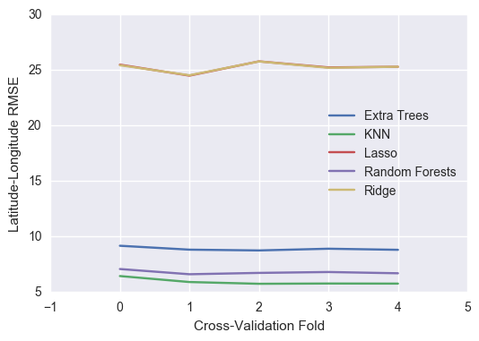
nested_crossval_results.plot()
plt.ylabel("Latitude-Longitude RMSE")
plt.xlabel("Cross-Validation Fold")
plt.xticks([-1,0,1,2,3,4,5])

([<matplotlib.axis.XTick at 0x11ffc8908>,
  <matplotlib.axis.XTick at 0x11143df60>,
  <matplotlib.axis.XTick at 0x10feb7080>,
  <matplotlib.axis.XTick at 0x10fce8860>,
  <matplotlib.axis.XTick at 0x111542cc0>,
  <matplotlib.axis.XTick at 0x1115427b8>,
  <matplotlib.axis.XTick at 0x10fb11f98>],
 <a list of 7 Text xticklabel objects>)

png

# First, let's save our data into a file
f = open("nested_crossval_global_results.pckl", "wb")
pickle.dump(nested_crossval_results,f)

4.5 Other Models

'''
# Support Vector Regression
pipe_svr = Pipeline([('scl', StandardScaler()),
            ('reg', MultiOutputRegressor(SVR()))])

grid_param_svr = {
    'reg__estimator__C': [0.01,0.1,1,10],
    'reg__estimator__epsilon': [0.1,0.2,0.3],
    'reg__estimator__degree': [2,3,4]
}

model_param_map[pipe_svr] = grid_param_svr

# Multi-Layer Perceptron
pipe_mlp = Pipeline([('scl', StandardScaler()),
            ('reg', MLPRegressor(random_state=1))])

grid_param_mlp = {
    'alpha': [0.0001,0.001,0.01,0.1],
    'learning_rate': ['constant','invscaling','adaptive']
}

model_param_map[pipe_mlp] = grid_param_mlp
'''

Based on the above nested cross-validation results, K Nearest Neighbors Regressor has the the lowest root mean square error for predicting latitude and longitude.

4.6 K Nearest Neighbors Hyper-Parameter Tuning

gs_knn = (GridSearchCV(estimator=pipe_knn,
                      param_grid=grid_param_knn,
                      cv=10,
                      scoring = 'neg_mean_squared_error',
                      n_jobs = 1))

gs_knn = gs_knn.fit(X_train,y_train)

gs_knn.best_estimator_

Pipeline(steps=[('scl', StandardScaler(copy=True, with_mean=True, with_std=True)), ('reg', KNeighborsRegressor(algorithm='auto', leaf_size=30, metric='manhattan',
          metric_params=None, n_jobs=-1, n_neighbors=3, p=2,
          weights='distance'))])

gs_knn_best = gs_knn.best_estimator_

gs_knn_best

Pipeline(steps=[('scl', StandardScaler(copy=True, with_mean=True, with_std=True)), ('reg', KNeighborsRegressor(algorithm='auto', leaf_size=30, metric='manhattan',
          metric_params=None, n_jobs=-1, n_neighbors=3, p=2,
          weights='distance'))])

gs_knn_best = Pipeline(steps=[('scl', StandardScaler(copy=True, with_mean=True, with_std=True)), ('reg', KNeighborsRegressor(algorithm='auto', leaf_size=30, metric='manhattan',
          metric_params=None, n_jobs=-1, n_neighbors=3, p=2,
          weights='distance'))])

knn_global_crossval = np.sqrt(np.abs((cross_val_score(estimator=gs_knn_best,
                                            X=X_train,
                                            y=y_train,
                                            cv=10,
                                            n_jobs=1,
                                            scoring = 'neg_mean_squared_error'))))

print('CV accuracy: %.3f +/- %.3f' % (np.mean(knn_global_crossval),
                                              np.std(knn_global_crossval)))

gs_knn_best.fit(X_train,y_train)

y_predict_train = gs_knn_best.predict(X_train)
err = np.sqrt(((y_train - y_predict_train)**2).sum(axis=1))
knn_global_train = np.sum(err, 0) / len(err)
print('Training RMSE: %.3f' % (knn_global_train))

y_predict_holdout = gs_knn_best.predict(X_test)
err = np.sqrt(((y_test - y_predict_holdout)**2).sum(axis=1))
knn_global_test = np.sum(err, 0) / len(err)     
print('Holdout RMSE: %.3f' % (knn_holdout_bf[key]))        

CV accuracy: 5.693 +/- 0.264
Training RMSE: 0.484
Holdout RMSE: 5.280

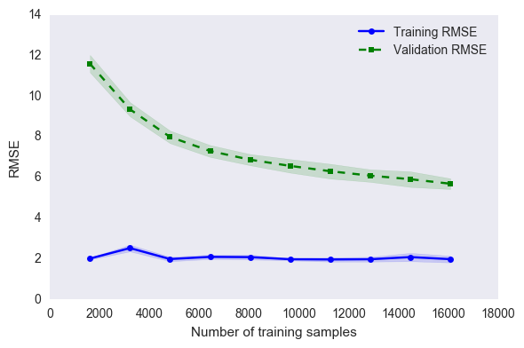
4.6.1 Learning Curve

## Credits: Sebastien's Python Machine Learning Book
train_sizes, train_scores, test_scores =\
                learning_curve(estimator=gs_knn_best,
                               X=X_train,
                               y=y_train,
                               train_sizes=np.linspace(0.1, 1.0, 10),
                               cv=10,
                               n_jobs=1,
                               scoring = 'neg_mean_squared_error'
                              )

train_scores = np.sqrt(np.abs(train_scores))
test_scores = np.sqrt(np.abs(test_scores))

train_mean = np.mean(train_scores, axis=1)
train_std = np.std(train_scores, axis=1)
test_mean = np.mean(test_scores, axis=1)
test_std = np.std(test_scores, axis=1)

plt.plot(train_sizes, train_mean,
         color='blue', marker='o',
         markersize=5, label='Training RMSE')

plt.fill_between(train_sizes,
                 train_mean + train_std,
                 train_mean - train_std,
                 alpha=0.15, color='blue')

plt.plot(train_sizes, test_mean,
         color='green', linestyle='--',
         marker='s', markersize=5,
         label='Validation RMSE')

plt.fill_between(train_sizes,
                 test_mean + test_std,
                 test_mean - test_std,
                 alpha=0.15, color='green')

plt.grid()
plt.xlabel('Number of training samples')
plt.ylabel('RMSE')
plt.legend(loc='upper right')
#plt.ylim([0.8, 1.0])
plt.tight_layout()
# plt.savefig('./figures/learning_curve.png', dpi=300)
plt.show()

png

5. Per-Building Per-Floor Regression

The goal is to tune the KNN model per-building per-floor.

5.1 Data Transformation

buildings = y_crossval.BUILDINGID.unique()
floors = y_crossval.FLOOR.unique()

buildings,floors

(array([2, 0, 1]), array([1, 3, 0, 2, 4]))

# bf indicates building-floor

X_crossval_bf = {}
y_crossval_bf = {}
X_holdout_bf = {}
y_holdout_bf = {}

for building in buildings:
    for floor in floors:

        # Finding index of samples with the building and floor

        index_crossval_bf = y_crossval[(y_crossval.BUILDINGID == building) & (y_crossval.FLOOR == floor)].index
        index_holdout_bf = y_holdout[(y_holdout.BUILDINGID == building) & (y_holdout.FLOOR == floor)].index

        if len(index_crossval_bf) == 0:
            continue

        key = (building,floor)

        X_crossval_bf[key] = X_pca_crossval.loc[index_crossval_bf]
        y_crossval_bf[key] = y_crossval.loc[index_crossval_bf,['LATITUDE','LONGITUDE']]

        X_holdout_bf[key] = X_pca_holdout.loc[index_holdout_bf]
        y_holdout_bf[key] = y_holdout.loc[index_holdout_bf,['LATITUDE','LONGITUDE']]

        print("Building = {}, Floor = {}".format(building,floor))
        print("Crossval shape", len(index_crossval_bf))
        print("Holdout shape", len(index_holdout_bf))

X_crossval_bf.keys(), X_holdout_bf.keys()

Building = 2, Floor = 1
Crossval shape 1950
Holdout shape 211
Building = 2, Floor = 3
Crossval shape 2420
Holdout shape 289
Building = 2, Floor = 0
Crossval shape 1725
Holdout shape 181
Building = 2, Floor = 2
Crossval shape 1405
Holdout shape 171
Building = 2, Floor = 4
Crossval shape 1011
Holdout shape 91
Building = 0, Floor = 1
Crossval shape 1220
Holdout shape 136
Building = 0, Floor = 3
Crossval shape 1247
Holdout shape 144
Building = 0, Floor = 0
Crossval shape 942
Holdout shape 116
Building = 0, Floor = 2
Crossval shape 1295
Holdout shape 148
Building = 1, Floor = 1
Crossval shape 1341
Holdout shape 143
Building = 1, Floor = 3
Crossval shape 825
Holdout shape 86
Building = 1, Floor = 0
Crossval shape 1239
Holdout shape 129
Building = 1, Floor = 2
Crossval shape 1254
Holdout shape 142





(dict_keys([(0, 1), (1, 2), (0, 0), (0, 2), (2, 1), (2, 4), (2, 0), (1, 3), (2, 3), (2, 2), (1, 0), (0, 3), (1, 1)]),
 dict_keys([(0, 1), (1, 2), (0, 0), (0, 2), (2, 1), (2, 4), (2, 0), (1, 3), (2, 3), (2, 2), (1, 0), (0, 3), (1, 1)]))

5.2 KNN Local

knn_local_crossval_bf = {}
knn_local_train_bf = {}
knn_local_holdout_bf = {}
knn_global_train_bf = {}
knn_global_holdout_bf = {}

for key in X_crossval_bf:
    print("Building = {}, Floor = {}".format(key[0],key[1]))

    X_train_bf = X_crossval_bf[key]
    y_train_bf = y_crossval_bf[key]

    X_test_bf = X_holdout_bf[key]
    y_test_bf = y_holdout_bf[key]

    model = Pipeline(steps=[('scl', StandardScaler(copy=True, with_mean=True, with_std=True)),
                                ('reg', KNeighborsRegressor(algorithm='auto', leaf_size=30, metric='manhattan',
                                                            metric_params=None, n_jobs=-1, n_neighbors=3, p=2,
                                                            weights='distance'))])
    model.fit(X_train_bf,y_train_bf)

    knn_local_crossval_bf[key] = np.sqrt(np.abs((cross_val_score(estimator=model,
                                            X=X_train_bf,
                                            y=y_train_bf,
                                            cv=5,
                                            n_jobs=1,
                                            scoring = 'neg_mean_squared_error'))))

    print('CV accuracy: %.3f +/- %.3f' % (np.mean(knn_local_crossval_bf[key]),
                                              np.std(knn_local_crossval_bf[key])))

    # Local KNN RMSE
    y_predict_train = model.predict(X_train_bf)
    err = np.sqrt(((y_train_bf - y_predict_train)**2).sum(axis=1))
    knn_local_train_bf[key] = np.sum(err, 0) / len(err)
    #print('Local Training RMSE: %.3f' % (knn_local_train_bf[key]))

    y_predict_holdout = model.predict(X_test_bf)
    err = np.sqrt(((y_test_bf - y_predict_holdout)**2).sum(axis=1))
    knn_local_holdout_bf[key] = np.sum(err, 0) / len(err)     
    #print('Local Holdout RMSE: %.3f' % (knn_local_holdout_bf[key]))

    # Global KNN RMSE
    y_predict_train = gs_knn_best.predict(X_train_bf)
    err = np.sqrt(((y_train_bf - y_predict_train)**2).sum(axis=1))
    knn_global_train_bf[key] = np.sum(err, 0) / len(err)
    #print('Global Training RMSE: %.3f' % (knn_global_train_bf[key]))

    y_predict_holdout = gs_knn_best.predict(X_test_bf)
    err = np.sqrt(((y_test_bf - y_predict_holdout)**2).sum(axis=1))
    knn_global_holdout_bf[key] = np.sum(err, 0) / len(err)     
    #print('Global Holdout RMSE: %.3f' % (knn_global_holdout_bf[key]))

Building = 0, Floor = 1
CV accuracy: 4.522 +/- 0.240
Building = 1, Floor = 2
CV accuracy: 5.263 +/- 0.362
Building = 0, Floor = 0
CV accuracy: 5.692 +/- 0.613
Building = 0, Floor = 2
CV accuracy: 4.465 +/- 0.435
Building = 2, Floor = 1
CV accuracy: 5.326 +/- 0.369
Building = 2, Floor = 4
CV accuracy: 8.174 +/- 0.816
Building = 2, Floor = 0
CV accuracy: 6.042 +/- 0.478
Building = 1, Floor = 3
CV accuracy: 7.333 +/- 0.625
Building = 2, Floor = 3
CV accuracy: 3.922 +/- 0.346
Building = 2, Floor = 2
CV accuracy: 4.969 +/- 0.589
Building = 1, Floor = 0
CV accuracy: 4.864 +/- 0.282
Building = 0, Floor = 3
CV accuracy: 4.338 +/- 0.250
Building = 1, Floor = 1
CV accuracy: 6.775 +/- 0.447

knn_local_crossval_bf = pd.Series(knn_local_crossval_bf)
knn_metric_df = (pd.concat([knn_local_crossval_bf.apply(np.mean),
                            knn_local_crossval_bf.apply(np.std),
                            pd.Series(knn_local_train_bf),
                            pd.Series(knn_local_holdout_bf),
                            pd.Series(knn_global_train_bf),
                            pd.Series(knn_global_holdout_bf)],axis=1))

knn_metric_df.columns = ['LOCAL_CROSSVAL_MEAN','LOCAL_CROSSVAL_STD',
                         'LOCAL_TRAINING_RMSE','LOCAL_HOLDOUT_RMSE',
                         'GLOBAL_TRAINING_RMSE','GLOBAL_HOLDOUT_RMSE']
knn_metric_df = knn_metric_df.rename_axis(['BUILDING','FLOOR'])

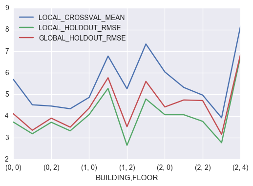
knn_metric_df[['LOCAL_CROSSVAL_MEAN','LOCAL_HOLDOUT_RMSE','GLOBAL_HOLDOUT_RMSE']].plot()

<matplotlib.axes._subplots.AxesSubplot at 0x120a75668>

png

# First, let's save our data into a file
f = open("knn_metric_df.pckl", "wb")
pickle.dump(knn_metric_df,f)

5.4 Best Local Model

pipe_knn = Pipeline([('scl', StandardScaler()),
            ('reg', KNeighborsRegressor(n_neighbors=3,
                                        metric='manhattan',
                                        weights = 'distance'))])

# Random Forests
reg_rf = RandomForestRegressor(random_state=1, n_estimators=50)

# Extra Trees
reg_et = ExtraTreesRegressor(random_state=1,n_estimators=50)

regs = [pipe_knn,reg_rf,reg_et]
reg_labels = ['KNN','Random Forests','Extra Trees']

reg_dict = dict(zip(reg_labels, regs))

best_local_crossval_bf = {}
best_local_train_bf = {}
best_local_holdout_bf = {}
best_local_model = {}

for key in X_crossval_bf:
    print("Building = {}, Floor = {}".format(key[0],key[1]))

    X_train_bf = X_crossval_bf[key]
    y_train_bf = y_crossval_bf[key]

    X_test_bf = X_holdout_bf[key]
    y_test_bf = y_holdout_bf[key]

    min_rmse= 1000

    for reg_label in reg_dict:
        model = reg_dict[reg_label]

        crossval_score = np.sqrt(np.abs((cross_val_score(estimator=model,
                                            X=X_train_bf,
                                            y=y_train_bf,
                                            cv=5,
                                            n_jobs=1,
                                            scoring = 'neg_mean_squared_error'))))

        if np.mean(crossval_score) < min_rmse:
            best_local_model[key] = reg_label
            best_local_crossval_bf[key] = crossval_score

    print('CV accuracy: %.3f +/- %.3f' % (np.mean(best_local_crossval_bf[key]),
                                              np.std(best_local_crossval_bf[key])))

    # Best RMSE
    best_model = reg_dict[best_local_model[key]]
    best_model.fit(X_train_bf,y_train_bf)

    y_predict_train = best_model.predict(X_train_bf)
    err = np.sqrt(((y_train_bf - y_predict_train)**2).sum(axis=1))
    best_local_train_bf[key] = np.sum(err, 0) / len(err)
    #print('Local Training RMSE: %.3f' % (knn_local_train_bf[key]))

    y_predict_holdout = best_model.predict(X_test_bf)
    err = np.sqrt(((y_test_bf - y_predict_holdout)**2).sum(axis=1))
    best_local_holdout_bf[key] = np.sum(err, 0) / len(err)     
    #print('Local Holdout RMSE: %.3f' % (knn_local_holdout_bf[key]))

Building = 0, Floor = 1
CV accuracy: 4.522 +/- 0.240
Building = 1, Floor = 2
CV accuracy: 5.263 +/- 0.362
Building = 0, Floor = 0
CV accuracy: 5.692 +/- 0.613
Building = 0, Floor = 2
CV accuracy: 4.465 +/- 0.435
Building = 2, Floor = 1
CV accuracy: 5.326 +/- 0.369
Building = 2, Floor = 4
CV accuracy: 8.174 +/- 0.816
Building = 2, Floor = 0
CV accuracy: 6.042 +/- 0.478
Building = 1, Floor = 3
CV accuracy: 7.333 +/- 0.625
Building = 2, Floor = 3
CV accuracy: 3.922 +/- 0.346
Building = 2, Floor = 2
CV accuracy: 4.969 +/- 0.589
Building = 1, Floor = 0
CV accuracy: 4.864 +/- 0.282
Building = 0, Floor = 3
CV accuracy: 4.338 +/- 0.250
Building = 1, Floor = 1
CV accuracy: 6.775 +/- 0.447

best_local_crossval_bf = pd.Series(best_local_crossval_bf)
best_local_metric_df = (pd.concat([pd.Series(best_local_model),
                                   best_local_crossval_bf.apply(np.mean),
                                   best_local_crossval_bf.apply(np.std),
                                   pd.Series(best_local_train_bf),
                                   pd.Series(best_local_holdout_bf)],
                                  axis=1))

best_local_metric_df.columns = ['BEST_LOCAL_MODEL','BEST_LOCAL_CROSSVAL_MEAN','BEST_LOCAL_CROSSVAL_STD',
                         'BEST_LOCAL_TRAINING_RMSE','BEST_LOCAL_HOLDOUT_RMSE']
best_local_metric_df = best_local_metric_df.rename_axis(['BUILDING','FLOOR'])

best_local_metric_df[['BEST_LOCAL_CROSSVAL_MEAN','BEST_LOCAL_TRAINING_RMSE','BEST_LOCAL_HOLDOUT_RMSE']].plot()

png

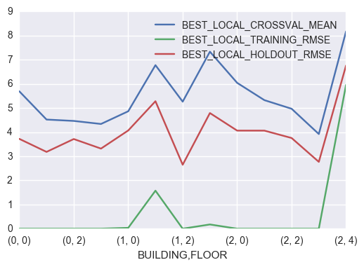
Interestingly, among the models compared, weighted KNN consistently has the minimum cross-validation RMSE independent of the building and floor.

# First, let's save our data into a file
f = open("best_local_metric_df.pckl", "wb")
pickle.dump(best_local_metric_df,f)

Share on

Twitter Facebook LinkedIn

Sharan Naribole