
Drawing Statistical Inferences from General Social Survey
25 minute read
In this project, I apply the skills learnt in Inferential Statistics course offered on Coursera by Duke University.
The R code used in this article is available on GitHub.
1. Introduction
With the General Social Survey dataset, I perform statistical inference tests to answer the following research topics:
Impact of News on Confidence in Government.
Income Disparity based on Citizenship.
Self-Employment Disparity between Genders.
Family Size impact on Financial Satisfaction.
Race representation among the Self-Employed.
I begin the project with the setup and dataset description. Then, for each research question posed above, I present the motivation, exploratory data analysis and the inferences drawn from statistical tests to answer the question.
2. Setup
2.1 Load packages
library(ggplot2)
library(dplyr)
library(statsr)
library(lattice)
2.2 Load data
Make sure your data and R Markdown files are in the same directory. When loaded your data file will be called gss. Delete this note when before you submit your work.
load("gss.Rdata")
2.3 Dataset Description
Source: GSS project description > Since 1972, the General Social Survey (GSS) has been monitoring societal change and studying the growing complexity of American society. The GSS aims to gather data on contemporary American society in order to monitor and explain trends and constants in attitudes, behaviors, and attributes; to examine the structure and functioning of society in general as well as the role played by relevant subgroups; to compare the United States to other societies in order to place American society in comparative perspective and develop cross-national models of human society; and to make high-quality data easily accessible to scholars, students, policy makers, and others, with minimal cost and waiting.
The survey has been conducted annually 1972-2012. For this project, I work with the Coursera extract of the raw survey dataset. In this extract, the missing values have been removed and few other modifications have been performed to make it convenient for practicing statistical reasoning using R. The extracted dataset consists of 57061 observations with 114 variables. Each variable corresponds to a specific question asked to the survey respondent. Expectedly, not every question is applicable to every respondent.
2.3.1 Scopes of Inference
As the survey is conducted by random sampling, the results from this project can be generalized to the entire US population. However, the statistical tests performed cannot provide causality relationships between the variables of interest.
3. Impact of News on Confidence in Government
3.1 Motivation
It has become a hot topic recently during the 2016 elections how fake news became widespread over the Internet and possibly led to voters forming strong political opinions. This motivates me to learn how the frequency of reading news might influenced the confidence one has in the executive branch of the government in earlier times.
3.2 Data
The variables analyzed in this study are:
news: A categorical variable indicating how often the respondent reads the newspaper.
conf: A categorical variable indicating whether the respondent has confidence in the executive branch of the government.
To reflect the latest trend in dependency between news reading and confidence in government, I focus on records in and after the year 2010. Let’s store only the above two variables for surveys on or after 2010. Also, let’s remove the records with missing values in either of the variables.
gss %>%
  filter(year >= 2010 &
           !is.na(news) &
           !is.na(confed)) %>%
  select(news,confed)  -> gss_news

dim(gss_news)
## [1] 1393 2
The dataset reduced to 1393 records from the total 57061 records.
3.3 Exploratory data analysis
table(gss_news$news, useNA = "ifany")
##
##          Everyday  Few Times A Week       Once A Week Less Than Once Wk
##               449               240               192               223
##             Never
##               289
Most of the respondents in our focused subset read the newspaper everyday.
table(gss_news$confed, useNA = "ifany")
##
## A Great Deal    Only Some   Hardly Any
##          200          644          549
Unsurprisingly, respondents with a great deal of confidence in the government are in the minority.
table(gss_news$news,gss_news$confed)
##
##                     A Great Deal Only Some Hardly Any
##   Everyday                    82       190        177
##   Few Times A Week            40       115         85
##   Once A Week                 30       101         61
##   Less Than Once Wk           24       116         83
##   Never                       24       122        143
g <- ggplot(data = gss_news, aes(x=news))
g <- g + geom_bar(aes(fill=confed), position = "dodge")
g + theme(axis.text.x = element_text(angle=60,hjust = 1))
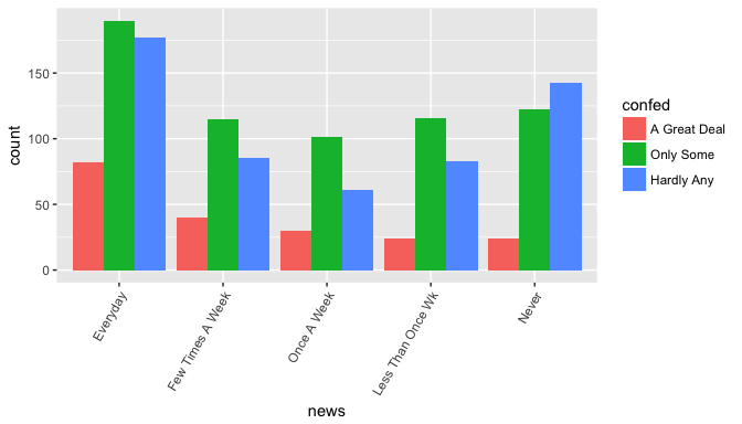
Observations:
Respondents with great deal of confidence are consistently lowest across all groups of news readers.
Respondents with only some confidence are majority across all groups except the respondents who never read the newspapers. Interestingly, responders who never read have majority with hardly any confidence in the executive branch of government.
Mosaic plots, a multi-dimension extension to the spine plots, provide a good illustration of the relationship between two categorical variables. The area of the tiles is proportional to the value counts within a group. When tiles across groups all have same areas, it indicates independence between the variables. Let’s plot it for our variables!
plot(table(gss_news$news,gss_news$confed))
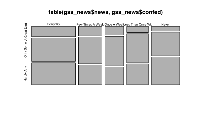
In the above mosaic plot, the area for the group A Great Deal monotonically decreases as the the frequency of reading decreases.
3.4 Inference
3.4.1 State Hypothesis
Null hypothesis: The frequency of reading newspapers and the confidence in the executive branch of the Government are independent.
Alternative hypothesis: The frequency of reading newspapers and the confidence in the executive branch of the Government are dependent.
3.4.2 Check Conditions
Independence: GSS dataset is generated from a random sample survey. We are fine in assuming that the records are independent.
Sample Size: As the samples are obtained without replacement, we must ensure they represent less than 10% of the population. The 1393 records we use for this analysis is indeed less than 10% of the total US population.
Degrees of Freedom: We have 3 confidence levels and 5 news reading frequency levels. As we have two categorical variables each with over 2 levels, we utilize the chi-squared test of independence to test the hypothesis.
Expected Counts: To perform a chi-square test (goodness of fit or independence), the expected counts for each cell should be at least 5. Let’s check that!
chisq.test(gss_news$news,gss_news$confed)$expected
##                    gss_news$confed
## gss_news$news       A Great Deal Only Some Hardly Any
##   Everyday              64.46518 207.57789  176.95693
##   Few Times A Week      34.45800 110.95477   94.58722
##   Once A Week           27.56640  88.76382   75.66978
##   Less Than Once Wk     32.01723 103.09548   87.88729
##   Never                 41.49318 133.60804  113.89878
From the above table, clearly every cell has an expected count more than 5. We’re now all clear to perform chi-squared test of independence! We will be using the inference function from the following link:
3.4.3 Chi-Squared test of independence
chisq.test(gss_news$news,gss_news$confed)
##
##  Pearson's Chi-squared test
##
## data:  gss_news$news and gss_news$confed
## X-squared = 32.728, df = 8, p-value = 6.895e-05
The chi-squared statistic is 32.728 and the corresponding p-value for 8 degrees of freedom is much lower than the significance level of 0.05.
3.5 Findings
We have convincing evidence to reject the null hypothesis in favor of the alternative hypothesis that the frequency of reading newspapers and confidence in the executive branch of the government are dependent. The study is observational, so we can only establish association but not causal links between these two variables.
4. Income Disparity based on Citizenship
4.1 Motivation
It is an ongoing debate that temporary workers from outside the U.S. are recruited by U.S. companies and paid much lower salaries than U.S. citizens. Although this debate has focused on the IT industry, comparing the total family incomes of U.S. Citizens and non-U.S. citizens in general and drawing statistical inferences would provide a better understanding.
4.2 Data
The variables used in this analysis are:
uscitzn: The respondent is either a) U.S. Citizen or b) not a U.S. citizen or c) U.S. citizen born in Puerto Rico, U.S. Virgin Islands, or the Northern Marianas Islands or d) Born outside the U.S. to parents who were U.S. citizens at that time or e) don’t know.
coninc: Inflation-adjusted family income. This would help us analyze the survey data across multiple years without worrying about the impact of inflation on the income.
Next, I select only the relevant variables and remove the missing values from the analysis.
gss %>%
  filter(!is.na(uscitzn) & !is.na(coninc)) %>%
  select(uscitzn,coninc)  -> gss_citzn

dim(gss_citzn)
## [1] 659 2
As the group names for uscitzn are too long, let’s create a shorter notation.
citzn_short <- function(word) {
  short = word

  if(short == "A U.S. Citizen Born In Puerto Rico, The U.S. Virgin Islands, Or The Northern Marianas Islands") {
    return("Islands")
  }
  if(short == "Born Outside Of The United States To Parents Who Were U.S Citizens At That Time (If Volunteered)") {
    return("Born Outside")
  }
  if(short == "A U.S. Citizen") {
    return("Citizen")
  }
  if(short == "Not A U.S. Citizen") {
    return("Not Citizen")
  }
}

gss_citzn$uscitzn = sapply(gss_citzn$uscitzn,citzn_short)

table(gss_citzn$uscitzn)
##
## Born Outside      Citizen      Islands  Not Citizen
##           10          315            5          329
We have less than or equal to 10 samples for each of the groups Islands and Born Outside.
4.3 Exploratory Data Analysis
ggplot(data=gss_citzn,aes(x=coninc)) + geom_histogram() + facet_wrap(~uscitzn)
## `stat_bin()` using `bins = 30`. Pick better value with `binwidth`.
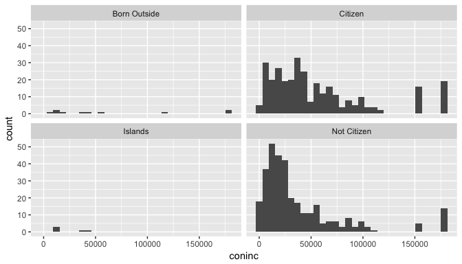
Observations:
Citizen and Not Citizen groups, our biggest groups have a right-skewed distribution.
The Islands groups has no samples with income above 50000.
4.4 Inference
4.4.1 State Hypothesis
Null hypothesis: The population mean of total family income with inflation correction is same for different U.S. citizen groups.
Alternative hypothesis: The population mean of total family income with inflation correction is different for at least one pair of U.S. citizen groups.
As we have more than 2 groups of citizenship, analysis of variance (ANOVA) is the right test to be conducted. First, we need to check if the necessary conditions to perform ANOVA test are satisfied or not.
4.4.2 Check Conditions
Independence: GSS dataset is generated from a random sample survey. We are fine in assuming that the records are independent within and across groups.
Nearly normal: To analyze the normality of the distributions, we can explore the quantile-quantile plot.
# 4 graphs in 2 rows
par(mfrow = c(2,2))
# Iterate on 4 groups and graph a QQ plot to test normality
citzn_groups = c("Citizen","Not Citizen","Islands","Born Outside")

for (i in 1:4) {
df = gss_citzn %>% filter(uscitzn == citzn_groups[i])
qqnorm(df$coninc, main=citzn_groups[i])
qqline(df$coninc)
}

Observations: There is a significant deviation from standard normal distribution in Citizen and Not Citizen groups especially in the upper quantile. This mirrors the right-skewed distributions we observed in the histogram plots.
- Variability: The variability across the groups needs to be about equal.
ggplot(data=gss_citzn,aes(x=uscitzn,y=coninc)) + geom_boxplot(aes(fill=uscitzn))
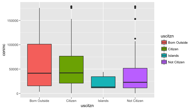
Observations: The variability across the groups varies significantly with the Born Outside group having the highest inter-quartile range. We observe the median for U.S Citizen group is much higher than that of non-U.S. citizens.
Based on the above observations, the conditions for performing ANOVA are not FULLY satisfied. Therefore, we need to be cautious in interpreting the results of ANOVA. Moreover, there might be external factors outside of citizenship that might be strongly correlated with income e.g. highest level of education.
4.4.3 ANOVA
anova(lm(coninc ~ uscitzn, data=gss_citzn))
## Analysis of Variance Table
##
## Response: coninc
##            Df     Sum Sq    Mean Sq F value    Pr(>F)
## uscitzn     3 5.8793e+10 1.9598e+10   9.791 2.521e-06 ***
## Residuals 655 1.3110e+12 2.0016e+09
With an f-statistic of 9.791 and p-value almost zero, we have strong evidence that at least one pair of the citizenship groups have different mean total inflation-corrected family income that cannot be explained simply by sampling variability. TO analyze which pair of groups have different incomes, we need to perform pairwise t-tests. One thing to keep in mind is that when we perform multiple comparisons, the chances of an extreme value that rejects the null hypothesis increases proportionally. To avoid this increase of Type 1 error rate (rejecting the null hypothesis when the null hypothesis is actually true), we incorporate the Bonferroni correction in the pairwise t-tests. With this correction, the significance level of each pairwise test α is reduced by k times where k is the number of pairwise tests.
Luckily, R comes with a simple function to perform the pairwise t-tests with the Bonferonni correction.
pairwise.t.test(gss_citzn$coninc, gss_citzn$uscitzn, p.adj="bonferroni")
##
##  Pairwise comparisons using t tests with pooled SD
##
## data:  gss_citzn$coninc and gss_citzn$uscitzn
##
##             Born Outside Citizen Islands
## Citizen     1.00         -       -
## Islands     0.50         0.59    -
## Not Citizen 0.35         2.4e-06 1.00
##
## P value adjustment method: bonferroni
Observations:
Interestingly, for most group pairs, p-value is much higher than 0.05/6, our reduced significance level.
With a p-value close to zero, we have strong evidence that the mean total inflation-corrected family income for U.S. Citizens and non U.S. Citizens is different and this difference cannot be explained by the sampling variability. We can be confident of this result because although ANOVA conditions weren’t satisfied, the sample size for both Citizen and Not Citizen groups is much higher than 30 and we can consider the sampling distribution of their difference to be nearly normal.
To dive further into analyzing these two groups, we need to filter out the other groups.
gss_citzn %>%
  filter(uscitzn == "Citizen" | uscitzn == "Not Citizen") -> gss_citzn_2group

dim(gss_citzn_2group)
## [1] 644 2
inference(y = coninc, x = uscitzn, data = gss_citzn_2group, statistic = "mean", type = "ci", conf_level = 0.95,method = "theoretical")
## Response variable: numerical, Explanatory variable: categorical (2 levels)
## n_Citizen = 315, y_bar_Citizen = 56156.254, s_Citizen = 47662.6977
## n_Not Citizen = 329, y_bar_Not Citizen = 38089.0213, s_Not Citizen = 41205.0202
## 95% CI (Citizen - Not Citizen): (11146.4694 , 24987.9959)
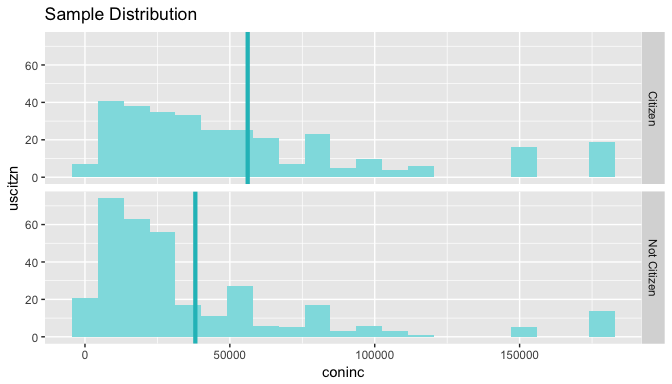
The 95% confidence interval for the mean total family income difference between U.S. Citizen and Non U.S. citizen groups is (11146.4694 , 24987.9959). As the value 0 is not present in this interval, the null hypothesis that these groups have the same mean family income would be rejected.
Findings
Although ANOVA conditions were not fulfilled, we observed through pairwise t-test that the mean total family income for U.S. Citizens and non U.S. Citizens were different. From exploratory data analysis, we observed the income to be higher for U.S. Citizen group. We are 95% confident that the mean difference between total inflation-corrected family income of U.S. citizens and non U.S. Citizens lies in the interval (11146.4694, 24987.9959) USD per annum.
5. Self-Employment Disparity between Genders
5.1 Motivation
With an exponential increase in the startups popping up all over the world, it is interesting to analyze if there are any differences between the two genders in entrepreneurship. For this purpose, I compare the proportions of men and women that are self-employed and draw statistical inferences.
5.2 Dataset
The variables used in this analysis are:
sex: A categorical variable indicating the gender of the respondent.
wrkslf: A categorical variable indicating whether the respondent is self-employed or works for someone else.
year: I expect the proportions to have increased across the years moving from 1972 to 2012.
gss %>%
  filter(!is.na(sex) & !is.na(wrkslf) & !is.na(year)) %>%
  select(sex,wrkslf,year) -> gss_gender_self

dim(gss_gender_self)
## [1] 53549 3
5.3 Exploratory Data Analysis
gss_gender_self %>%
  group_by(sex,year) %>%
  summarise(prop = sum(wrkslf == "Self-Employed")/n()) -> gss_gender_prop

ggplot(data=gss_gender_prop, aes(x=year,y=prop)) + geom_smooth(aes(fill=sex))
## `geom_smooth()` using method = 'loess' and formula 'y ~ x'
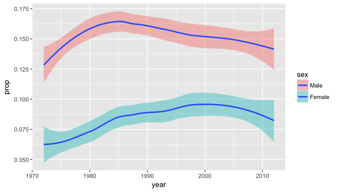
The above figure displays the loess regression curves for the self-employed proportion in men and women.
Observations:
Interestingly, the peak for men occurred around 1985 whereas the peak for women occurred much later in 1998.
Consistently, the proportion for men is higher than for women.
5.4 Inference
5.4.1 State Hypothesis
Null hypothesis: The mean difference in proportions of self-employed men and women is zero.
Alternate hypothesis: The mean difference in proportions of self-employed men and women is greater than zero.
To test the hypothesis, we perform the one-sided z-test test for two independent sample proportions.
5.4.2 Check Conditions
Independence: The observations in each group are independent from the random sampling conducted in GSS survey.
Sample size: To check the sample size, we need to find out first the pooled proportion $\hat{p}_{pool}$ which is expressed in this context as number of self-employed men and women / total number of men and women.
gss_gender_self %>%
  summarise(p_pool = sum(wrkslf=="Self-Employed")/n(),
            n_1 = sum(sex == "Female"),
            n_2 = sum(sex == "Male"),
            n_1_success = p_pool*n_1,
            n_1_fails = (1-p_pool)*n_1,
            n_2_success = p_pool*n_2,
            n_2_fails = (1-p_pool)*n_2,
            SE = sqrt((p_pool*(1 - p_pool)/n_1) + (p_pool*(1 - p_pool)/n_2)))
##      p_pool   n_1   n_2 n_1_success n_1_fails n_2_success n_2_fails
## 1 0.1157258 29031 24518    3359.635  25671.36    2837.365  21680.64
##            SE
## 1 0.002774666
From the above data, the minimum expected counts criterion of 10 is met for each cell in our 2x2 matrix. The distribution of the sample proportion will be nearly normal, centered at the true population mean.
#### 5.4.3 One-Sided Independent Sample Proportion t–test
inference(y = wrkslf, x = sex, data = gss_gender_self, statistic = "proportion", type = "ht", null = 0, success="Self-Employed", alternative ="greater", method = "theoretical")
## Response variable: categorical (2 levels, success: Self-Employed)
## Explanatory variable: categorical (2 levels)
## n_Male = 24518, p_hat_Male = 0.1525
## n_Female = 29031, p_hat_Female = 0.0847
## H0: p_Male =  p_Female
## HA: p_Male > p_Female
## z = 24.4198
## p_value = < 0.0001
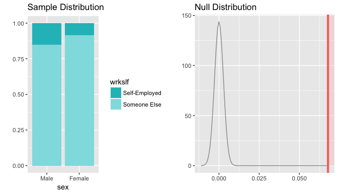
From the above result, the z-score indicates our observed difference in proportions is 24.198 standard deviations away from the mean in the null hypothesis. Clearly, with the p-value < 0.0001, the observed data cannot be explained by the sampling variability of our null hypothesis. We have convincing evidence that the proportion of self-employed men is greater than proportion of self-employed women in the U.S.
Findings
In the exploratory data analysis phase, we observed that the self-employed male proportion is consistently higher than the corresponding female proportions across all the years in the period 1972-2012. Through statistical test of two independent sample proportions, we obtain strong evidence of the higher proportion of self-employed in male respondents.
6. Family Size impact on Financial Satisfaction
6.1 Motivation
In this analysis, I am interested in finding out if the financial satisfaction of the respondents is impacted by the number of children in the family. My expectation is that the financial situation worsens with the number of children.
6.2 Dataset
The variables used in this analysis are:
childs: The number of children in the family. Eight or more children is censored to value of 8.
satfin: Categorical variable indicating the satisfaction with current financial situation.
By looking at the entire dataset of 1972-2012, we are removing impact of seasonal and event-specific factors that might influence our results when analysis shorter time periods. Also, we are interested in comparing the extreme cases of being Satisfied or Not at all Satisfied.
gss %>%
  filter(!is.na(childs) &
           !is.na(satfin) &
           !is.na(year) &
           satfin != "More Or Less") %>%
  select(childs,satfin,year) -> gss_satfin

dim(gss_satfin)
## [1] 29183 3
6.3 Exploratory Data Analysis
ggplot(data=gss_satfin,aes(x=year,y=childs)) + geom_smooth(aes(fill=satfin))
## `geom_smooth()` using method = 'gam' and formula 'y ~ s(x, bs = "cs")'
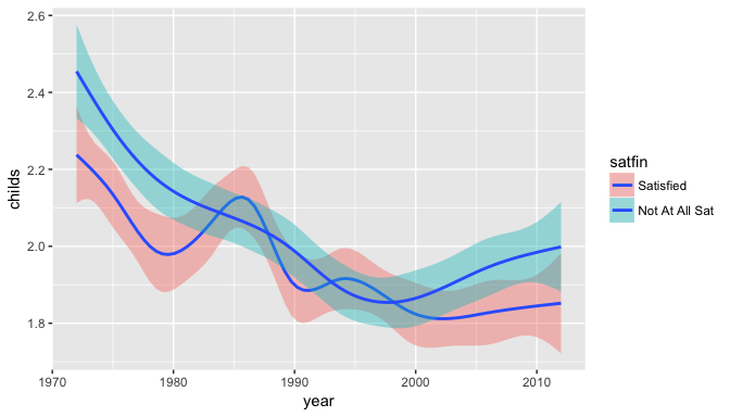
Observations:
Interestingly, the Not At All Satisfied group had a higher mean in the earlier period before 1985. Since 1998, it has again stayed at the top.
The Satisfied group experienced a local maximas at 1986 and 1995.
The reasons for these local maxima need to be investigated later. For the rest of this analysis, I consider the number of children as a categorical variable.
gss_satfin %>%
  mutate(childs = as.character(childs)) -> gss_satfin

plot(table(gss_satfin$childs,gss_satfin$satfin))
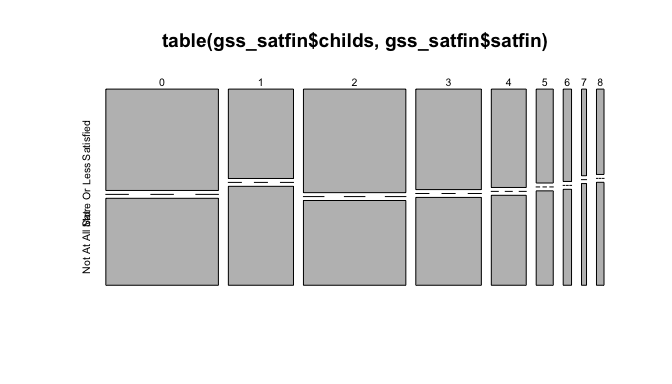
Observations:
- Initially, for number of children less than 6, we observe fairly equal proportions between the Satisfied and Not At All Satisfied groups.
- When the number of children is high, 8 or more, the proportion of Not at all Satisfied group is much larger.
6.4 Inference
6.4.1 State Hypothesis
Null hypothesis: The number of children and financial satisfaction are independent.
Alternative hypothesis: The number of children and financial satisfaction are dependent.
As we have two Satisfaction groups and 8 number of children groups, the hypothesis test to be performed is the chi-sq test of independence.
6.4.2 Check Conditions
Independence: The samples are independent as discussed previously in this article.
Expected Counts:
chisq.test(gss_satfin$childs,gss_satfin$satfin)$expected
##                  gss_satfin$satfin
## gss_satfin$childs Satisfied Not At All Sat
##                 0 4113.9809      3735.0191
##                 1 2380.6474      2161.3526
##                 2 3742.8892      3398.1108
##                 3 2395.8474      2175.1526
##                 4 1276.2828      1158.7172
##                 5  623.2034       565.7966
##                 6  304.5258       276.4742
##                 7  183.4493       166.5507
##                 8  275.1739       249.8261
From the above table, the expected counts are above the minimum required of 5 for each cell.
- Degrees of Freedom: The degrees of freedom is given by 8 (= (9-1)*(2-1)).
All the conditions to perform chi-square test of independence are satisfied.
6.4.3 Chi-Square test of independence
chisq.test(gss_satfin$childs,gss_satfin$satfin)
##
##  Pearson's Chi-squared test
##
## data:  gss_satfin$childs and gss_satfin$satfin
## X-squared = 93.573, df = 8, p-value < 2.2e-16
6.5 Findings
With a p-value of almost zero, we have strong evidence to reject the null hypothesis. Hence, we have convincing evidence to state that the number of children in a family and the financial satisfaction are dependent in the U.S.
7. Race representation among the Self-Employed
7.1 Motivation
In the last analysis of this project, I am interested in finding out if the people belonging to different races are proportionally represented among the self-employed.
7.2 Dataset
The variables used in this analysis are:
race: Categorical variable indicating white, black or other.
wrkslf: Indicating whether the respondent is self-employed or works for someone.
gss %>%
  filter(!is.na(race) & !is.na(wrkslf)) %>%
  select(race,wrkslf) -> gss_race

dim(gss_race)
## [1] 53549 2
7.3 Exploratory Data Analysis
Let’s try to find out the overall proportions of each race.
gss_race %>%
  group_by(race) %>%
  summarise(prop = n()/dim(gss_race)[1]) -> expected_prop

expected_prop
## # A tibble: 3 × 2
##     race       prop
##   <fctr>      <dbl>
## 1  White 0.81661656
## 2  Black 0.13600627
## 3  Other 0.04737717
Clearly, the White group has the leading percentage share out of all the races in our dataset.
Let’s find the expected counts among Self-Employed.
# Total Number of Self-Employed
Nself_employed = dim(gss_race %>% filter(wrkslf == "Self-Employed"))[1]

expected_prop %>%
  mutate(expected_counts = prop*Nself_employed) -> expected_prop

gss_race %>%
  filter(wrkslf == "Self-Employed") %>%
  group_by(race) %>%
  summarise(observed_counts = n()) -> final_df
final_df <- full_join(final_df,expected_prop,by="race")

final_df
## # A tibble: 3 × 4
##     race observed_counts       prop expected_counts
##   <fctr>           <int>      <dbl>           <dbl>
## 1  White            5477 0.81661656       5060.5728
## 2  Black             454 0.13600627        842.8309
## 3  Other             266 0.04737717        293.5963
Interestingly, there is a significant difference in the number of black respondents between the observed data and expected counts.
7.4 Inference
7.4.1 State Hypothesis
Null hypothesis: The distribution of self-employed follows the hypothesized distribution, and any observed differences are due to chance. The hypothesized distribution is the overall distribution of people belonging to different races.
Alternate hypothesis: The distribution of observed counts does not follow the hypothesized distribution.
To test the hypotheses, we have to perform the chi-square goodness of fit test. Let’s check if the conditions are satisfied.
7.4.2 Check Conditions
Independence: Yes, as discussed in previous research questions.
Expected counts: The expected count is above the minimum of 5 for each cell in our table.
Degrees of Freedom: The degree of freedom is equal to 2 (= 3-1).
All the conditions for performing chi-square goodness of fit test are satisfied.
7.4.2 Chi-Squared goodness of fit
chisq.test(x = final_df$observed_counts,p = final_df$prop)
##
##  Chi-squared test for given probabilities
##
## data:  final_df$observed_counts
## X-squared = 216.24, df = 2, p-value < 2.2e-16
Based on the p-value almost zero, we have strong evidence to reject the null hypothesis that the distribution of self-employed follows the hypothesized distribution. The observed counts cannot be explained by just the sampling variability of the null hypothesized distribution.
7.5 Finding
We obtained strong evidence that the people belonging to different races are not well-represented among the self-employed in U.S.
Conclusion
In this project, I utilized the General Social Survey Coursera Extract dataset to pose several research questions. Using statistical tests learnt in the Inferential Statistics offered on Coursera by Duke University, I drew statistical inferences for each research question that can be generalized to the entire U.S. population.
The code used in this article is available on GitHub. Thanks for reading!
References
Citation for the original dataset:
Smith, Tom W., Michael Hout, and Peter V. Marsden. General Social Survey, 1972-2012 [Cumulative File]. ICPSR34802-v1. Storrs, CT: Roper Center for Public Opinion Research, University of Connecticut /Ann Arbor, MI: Inter-university Consortium for Political and Social Research [distributors], 2013-09-11. <doi:10.3886/ICPSR34802.v1> Persistent URL: http://doi.org/10.3886/ICPSR34802.v1