
Stock Return Classifier (Part I): Problem Statement & Technical Indicators
7 minute read
This post is part of a series on building a supervised ML pipeline to classify SPY daily returns.
- Part I: Problem Statement & Technical Indicators
- Part II: EDA, Feature Selection & Feature Engineering
- Part III: Baseline Models, ML Models & Hyperparameter Tuning
- Part IV: Test Evaluation & Portfolio Backtesting
Next Post → Part II: EDA, Feature Selection & Feature Engineering
⚠️ Disclaimer
This blog series is for educational and research purposes only. The content should not be considered financial advice, investment advice, or trading advice. Trading stocks and financial instruments involves substantial risk of loss and is not suitable for every investor. Past performance does not guarantee future results. Always consult with a qualified financial advisor before making investment decisions.
Introduction
After completing the DQN Trading series, I wanted to revisit the same SPY prediction problem through a supervised learning lens. Reinforcement learning directly optimises a trading policy—but can a simpler binary classifier reliably identify high-return days before they happen?
This series documents building a complete ML pipeline to predict whether SPY (the S&P 500 ETF) will gain ≥ 1% in a single trading day. The pipeline covers data collection, feature engineering, EDA, model training, temporal cross-validation, and portfolio backtesting on a held-out 2-year test period.
The complete code is available on GitHub.
Problem Statement
The Classification Task
Objective: Predict whether SPY will close ≥ 1% higher than the current day’s close.
target[t] = 1  if  (Close[t+1] - Close[t]) / Close[t]  >=  1.0%
           = 0  otherwise
This is a binary classification problem with a clear economic interpretation: a positive prediction signals a buy opportunity—deploy capital today, collect the gain tomorrow.
The 1% threshold is deliberate. It filters out noise and transaction-cost territory, targeting only days with meaningful upside. This creates a challenging but practical task: such days are relatively rare, making class imbalance a central design concern (covered in Part II).
Why SPY?
SPY is the world’s most traded ETF—tracking the S&P 500 index with tight bid-ask spreads and deep liquidity. For a backtesting exercise, SPY has several advantages:
- Reliable adjusted data:
auto_adjust=Truefrom yfinance gives price-continuous adjusted close, high, and low—consistent across splits and dividends - No survivorship bias: The index reconstitutes over time; SPY captures that in a single liquid instrument
- Market-wide signal: SPY moves on macro and sector-level forces, making technical indicators more interpretable than for individual stocks
- Historical depth: 20+ years of reliable daily data (we use 2006 to present)
Why Supervised Classification?
Unlike the DQN approach—where the agent learns a full trading policy—supervised classification focuses on a single, well-defined prediction: will tomorrow be a big up day?
This simplicity has advantages:
- Interpretability: Standard classification metrics (precision, recall, F1, AUC-ROC) directly measure prediction quality
- Temporal cross-validation: Expanding-window CV gives honest, fold-by-fold estimates of generalisation
- Portfolio strategies: Once we have calibrated probabilities, multiple trading strategies can be evaluated without retraining
The tradeoff is that the classifier doesn’t model the full hold/sell decision loop—that remains the domain of RL agents. But for the specific question of “when to buy”, a well-calibrated classifier can be surprisingly effective.
Pipeline Overview
The project is structured as a sequence of seven standalone notebooks, each reading from files produced by the previous stage:
| # | Notebook | Output |
|---|---|---|
| 01 | Data Collection | data/raw/{project}_raw.parquet |
| 02 | Data Preprocessing | 22 features added, target created, temporal splits, normalization |
| 03 | EDA | Distribution plots, MI scores → eda_recommendations.json |
| 04 | Feature Engineering | Log1p transforms, redundant features dropped |
| 05 | Baseline Models | Majority-class and MACD momentum benchmarks |
| 06 | ML Models | HPT, learning curves, model selection, best_model.pkl |
| 07 | Test Evaluation | Confusion matrix, ROC, calibration, portfolio simulation |
Two JSON configs control every experiment—data_config.json (ticker, date range, splits) and model_config.json (models, hyperparameters, portfolio settings)—by setting PROJECT_FOLDER at the top of each notebook.
Data Collection
Sources
Two data sources are combined:
- SPY OHLCV — adjusted open, high, low, close, volume from Yahoo Finance (
auto_adjust=True) - VIX — CBOE Volatility Index close (ticker
^VIX)
Both are downloaded via yfinance with smart CSV caching: the cache filename encodes the full date range ({TICKER}_{YYYYMMDD}_{YYYYMMDD}.csv), so subsequent runs reuse cached data if the range is already covered. A 60-day warm-up buffer prepends the requested start date to ensure all indicators have enough historical context on day one.
Date Range
The spy_run config uses:
- Start: 2006-01-01 (with 60-day buffer prepended)
- End: auto (yesterday’s close)
- Test period: last 2 years held out (Feb 2024 – Feb 2026 in the current run)
Technical Indicators
All 22 features are computed in src/features/engineer.py using the ta library. They span four categories:
Volatility
| Feature | Description |
|---|---|
BB_High, BB_Low | Bollinger Bands (20-day, 2σ) |
BB_Width | (BB_High − BB_Low) / BB_Mid — band squeeze proxy |
BB_Position | (Close − BB_Low) / (BB_High − BB_Low) — price within band |
ATR_pct | ATR / Close × 100 — scale-invariant daily range |
BB_Position is a normalised indicator ranging 0–1: values near 0 indicate the price is near the lower band (potential oversold), values near 1 indicate proximity to the upper band (potential overbought). BB_Width captures the “squeeze” pattern—bands contracting often precede breakouts.
Trend
| Feature | Description |
|---|---|
EMA_8, EMA_21 | Short and medium exponential moving averages |
ADX | Average Directional Index (14-day) — trend strength |
EMA crossovers and ADX are classic trend-following signals. ADX above 25 conventionally indicates a trending (vs. ranging) market.
Momentum
| Feature | Description |
|---|---|
RSI | Relative Strength Index (14-day) |
MACD_line, MACD_signal, MACD_hist | 12/26 MACD and 9-day signal line |
Stoch_K, Stoch_D | Stochastic %K (14-day) and %D (3-day smooth) |
ROC_3, ROC_5 | 3-day and 5-day rate of change |
Price_Return_1, Price_Return_5 | 1-day and 5-day percentage return |
IBS | Intra-Bar Strength: (Close − Low) / (High − Low) |
IBS is a lesser-known but effective mean-reversion indicator. Days with IBS near 0 (close at day low) have historically preceded rebounds; days near 1 (close at day high) have preceded pullbacks in mean-reverting regimes.
Market Regime
| Feature | Description |
|---|---|
VIX_Close | CBOE Volatility Index — market fear/regime |
Volume | Daily share volume |
VIX is arguably the single most informative macro feature. High VIX periods (market stress) tend to produce both more frequent ≥1% up days and more frequent large drawdowns—making it an important regime signal.
Time Series Visualisation
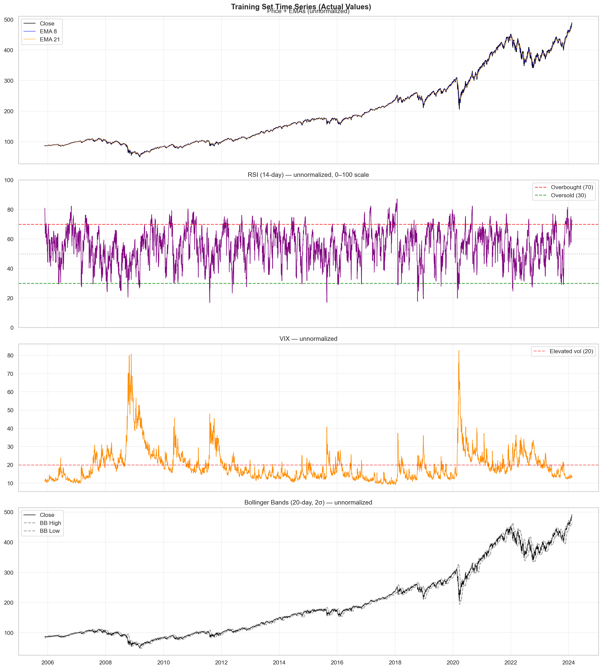
The time series plot shows SPY adjusted close alongside key indicators computed from 2006 to present. The price action, Bollinger Bands, RSI, and VIX are plotted together to visualise how market conditions vary across the full training history. Periods of high VIX correspond to increased volatility and potential ≥1% day frequency—most visibly around the 2008–2009 financial crisis, the 2020 COVID crash, and 2022 rate-hike drawdown.
Normalisation Strategy
Raw feature values are not directly fed to the models. Two normalisation strategies are supported:
Rolling Z-score (default):
z[t] = (x[t] - mean(x[t-W : t])) / std(x[t-W : t])
With a 63-day backward window (roughly one trading quarter), this normalises each feature relative to its recent distribution. This is computed on the continuous timeline before splitting—using only backward-looking windows at every point, so no future information leaks into any training fold.
Standard scaler: StandardScaler fit on the training split only, then applied to validation and test. Binary features (Market_Trend, any 0/1 indicator) are excluded from normalisation in both approaches.
What’s Next?
In Part II, we’ll explore the data and select the features that matter:
- Class distribution and imbalance quantification
- Feature distributions and skewness analysis
- Correlation heatmap and mutual information scores
- EDA-driven feature engineering: log1p transforms and redundant feature removal
Next Post → Part II: EDA, Feature Selection & Feature Engineering
References
- yfinance Documentation - Yahoo Finance API wrapper
- Technical Analysis Library in Python (ta)
- Bollinger Bands - Investopedia
- RSI Indicator Guide - Investopedia
- MACD Indicator - Investopedia
- VIX Index Overview - CBOE