
Stock Return Classifier (Part IV): Test Evaluation & Portfolio Backtesting
12 minute read
This post is part of a series on building a supervised ML pipeline to classify SPY daily returns.
- Part I: Problem Statement & Technical Indicators
- Part II: EDA, Feature Selection & Feature Engineering
- Part III: Baseline Models, ML Models & Hyperparameter Tuning
- Part IV: Test Evaluation & Portfolio Backtesting
← Previous: Part III: Baseline Models, ML Models & Hyperparameter Tuning
⚠️ Disclaimer
This blog series is for educational and research purposes only. The content should not be considered financial advice, investment advice, or trading advice. Trading stocks and financial instruments involves substantial risk of loss and is not suitable for every investor. Past performance does not guarantee future results. Always consult with a qualified financial advisor before making investment decisions.
Introduction
In Part III, we selected Random Forest as the best model based on ROC-AUC tiebreak among models with similar F1 scores. Now we evaluate it on the held-out test set—502 trading days from February 2024 to February 2026—data the model has never seen.
This is the moment of truth: validation scores are honest, but they reflect the past. Test evaluation tells us whether the patterns learned generalise to the most recent 2 years of market data.
Test Set: 502 Trading Days
The test period (Feb 2024 – Feb 2026) represents a challenging evaluation environment:
- SPY experienced multiple significant drawdowns and recoveries
- VIX spiked several times above 20 during tariff/geopolitical uncertainty
- The period includes both the 2024 rally and subsequent volatility in early 2025
All test predictions use the model trained on the full 2006–Feb 2024 training set with the best hyperparameters found in Part III.
Classification Metrics
Confusion Matrix
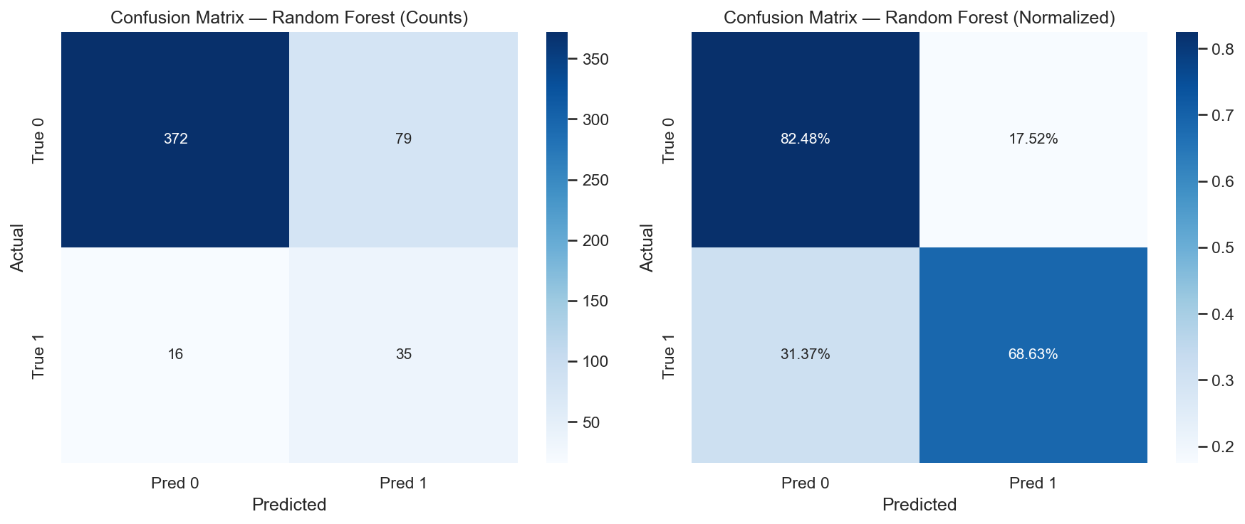
Left: raw counts. Right: row-normalised percentages. The model correctly identifies ~69% of actual up days (high recall) with 30.7% precision. The normalised view makes class-level error rates directly comparable despite the imbalance.
| Metric | Value |
|---|---|
| Accuracy | 0.811 |
| Precision | 0.307 |
| Recall | 0.686 |
| F1 | 0.424 |
| ROC-AUC | 0.812 |
Recall of 0.686 means the model catches roughly 69% of the actual ≥1% up days in the test period.
Precision of 0.307 means that of the buy signals generated, about 31% correspond to actual ≥1% up days. The remaining signals trade on days that don’t hit the 1% threshold—though many of these are profitable at smaller gains (addressed in the portfolio section below).
AUC-ROC of 0.812 is the headline metric: the model correctly ranks a randomly chosen positive day above a randomly chosen negative day 81% of the time. This is strong ranking performance for daily return prediction.
ROC Curve
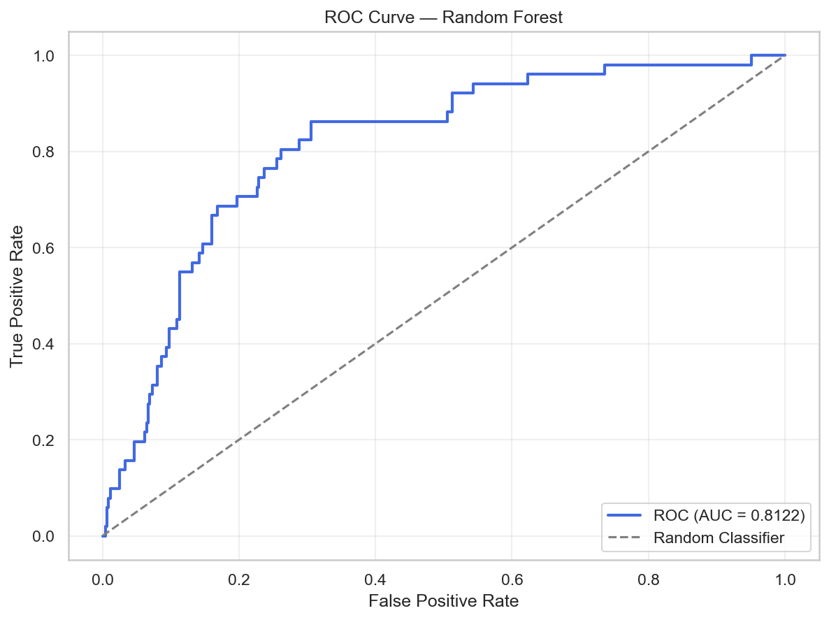
AUC of 0.812 on the held-out test set (vs. 0.722 at validation) indicates the model generalises well—and actually improves on test. This reflects the fact that expanding window validation uses earlier historical folds that may be less representative of current market dynamics. The test period’s market conditions appear well-captured by the full training history.
The validation AUC (0.722) vs. test AUC (0.812) gap is worth noting. While this direction (test > val) can sometimes indicate lucky test period selection, it also reflects expanding window validation averaging across folds of varying quality—earlier folds train on less data and may underperform.
Precision vs. Win Rate
An important distinction in the portfolio context:
- Precision (30.7%): Among all buy signals, ~31% hit the ≥1% threshold—the specific target the classifier was trained on.
- Win rate (~64%): Among all trades executed, ~64% close at a higher price than entry (next-day close > entry close).
These measure different things. Precision reflects the classification objective. Win rate reflects raw profitability at any positive return level. The gap between 30.7% and 64% means many signals—while not meeting the ≥1% classification target—still produce profitable trades.
Calibration
A well-calibrated classifier’s predicted probability of class 1 should match the actual fraction of positives at each probability level. If the model says 60% probability, approximately 60% of those days should be genuine ≥1% up days.
The calibration curve shows moderate miscalibration at the extremes—the model slightly overestimates probabilities in the mid-range. This matters for Strategy 2 and Strategy 3, which use probability thresholds to control position sizing. Well-calibrated probabilities ensure the thresholds have their intended meaning.
Portfolio Backtesting
Classification metrics tell us how good the predictions are. Portfolio simulation translates predictions into economic outcomes.
Setup
- Initial balance: $100,000
- Hold period: 1 day (buy at close, sell at next close)
- Position sizing: deploy maximum affordable shares on each signal (balance-based)
- No transaction costs (SPY has near-zero bid-ask spread for large accounts)
The 1-day hold period matches the prediction horizon exactly: we predicted whether tomorrow will be a ≥1% day, so we hold for exactly 1 day.
Three ML Strategies
Strategy 1: Buy max affordable shares whenever prob > 0.5. Most aggressive—fires on any net-positive signal.
Strategy 2: Buy max affordable shares whenever prob ≥ 0.6. Higher confidence threshold—fires less often but with more conviction.
Strategy 3: Variable position sizing by probability bin:
| Probability | Position Size |
|---|---|
| ≥ 0.875 | 100% of max affordable |
| 0.75 – 0.875 | 75% |
| 0.625 – 0.75 | 50% |
| 0.50 – 0.625 | 25% |
Strategy 3 scales exposure proportionally with the model’s conviction. Lower-confidence signals deploy only a fraction of available capital, reducing risk on uncertain trades while still participating in the upside.
Baseline Strategies
To contextualise the ML strategies, we compare against three non-ML approaches:
MACD Strategy: Buy max affordable shares whenever MACD histogram > 0, sell 1 day later—the same hold period as the ML strategies. This is the portfolio equivalent of the MACD classification baseline from Part III, testing whether a single-indicator rule can match ML-driven signals.
DCA Weekly: Split the initial $100K into equal portions and invest one portion every 5 trading days, buying and holding until the end of the test period. Pure accumulation with no selling between intervals.
DCA Monthly: Same as DCA Weekly but investing every 21 trading days—fewer but larger purchases.
DCA strategies provide a passive investment baseline. They require zero prediction skill and represent the “just buy regularly” approach that any active strategy must justify itself against.
Portfolio Results
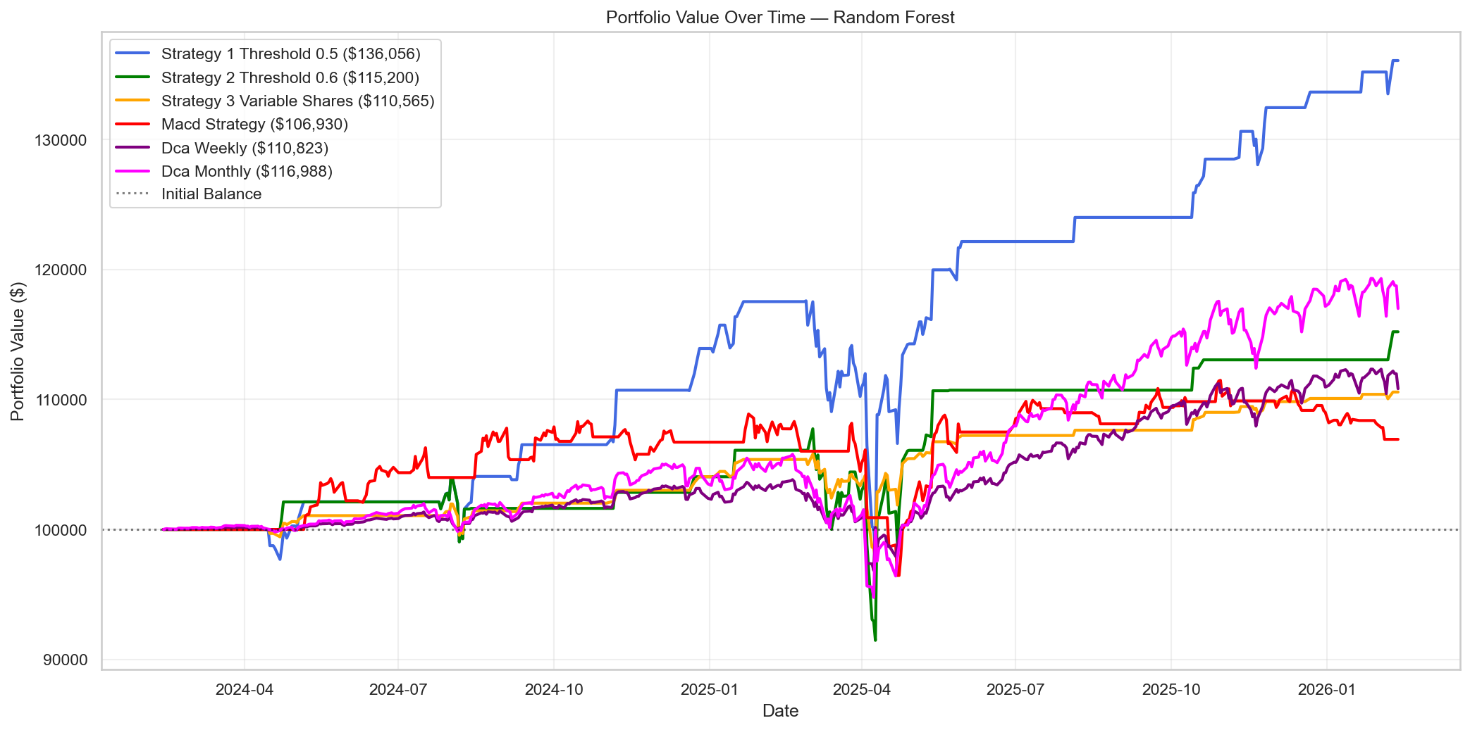
All strategies start at $100,000 and are tracked daily across the 502-day test period. Strategy 1 dominates with +36.06% return and the highest Sharpe ratio (1.099). All ML strategies outperform the MACD rule-based approach. DCA Monthly provides a strong passive baseline but Strategy 1 still exceeds it by a wide margin.
| Strategy | Return | Final Value | Sharpe | Max Drawdown | Trades | Win Rate |
|---|---|---|---|---|---|---|
| Strategy 1 (prob > 0.5) | +36.06% | $136,056 | 1.099 | -16.24% | 114 | 64.0% |
| Strategy 2 (prob ≥ 0.6) | +15.20% | $115,200 | 0.486 | -15.10% | 63 | 63.5% |
| Strategy 3 (variable sizing) | +10.57% | $110,565 | 0.547 | -7.57% | 114 | 64.0% |
| MACD Strategy | +6.93% | $106,930 | 0.206 | -11.40% | 227 | 56.8% |
| DCA Weekly | +10.82% | $110,823 | 0.578 | -6.72% | 101 | 91.1% |
| DCA Monthly | +16.99% | $116,988 | 0.705 | -10.40% | 24 | 95.8% |
Analysis
Strategy 1 dominates across the board:
Strategy 1 outperforms every baseline on both raw return and Sharpe ratio:
- vs. MACD: +29.13 pp return, 5.3× higher Sharpe
- vs. DCA Monthly: +19.07 pp return, 1.56× higher Sharpe
- vs. DCA Weekly: +25.24 pp return, 1.90× higher Sharpe
The Sharpe ratio of 1.099 is the most meaningful result. It shows the model adds value not just by capturing more returns, but by doing so with favourable risk-adjusted characteristics.
Why does Strategy 1 beat passive approaches?
DCA strategies are permanently accumulating and holding—they participate in every down day once invested. Strategy 1 holds for only 1 day at a time and is in cash the rest. When in cash, it avoids prolonged drawdown periods. However, this selectivity comes with execution risk: missing a few large up days could erase the advantage.
Strategy 3 achieves the lowest ML drawdown:
At -7.57% max drawdown, Strategy 3 offers the best risk management among the ML strategies. By deploying only 25% of capital on lower-confidence signals (0.50–0.625), it limits exposure on uncertain predictions. The tradeoff is a much lower total return (+10.57% vs. +36.06%).
Strategy 2 underperforms:
At the 0.6 threshold, Strategy 2 generates only 63 signals vs. 114 for Strategy 1. The reduced trade frequency cuts the number of winning trades proportionally, leading to lower total return (+15.20%). The 0.6 threshold is too restrictive given the model’s calibration: most of the model’s useful signals fall in the 0.5–0.6 probability range.
MACD Strategy is the weakest:
Despite trading the most frequently (227 trades), the MACD strategy achieves only +6.93% return with a 56.8% win rate. The single-indicator rule fires too indiscriminately—it can’t distinguish between genuine ≥1% up days and ordinary positive-momentum days. This confirms the value of multi-feature ML models over single-indicator rules.
Win Rate vs. Precision revisited:
Strategy 1 achieves a 64% win rate despite precision of only 30.7%. This confirms the earlier observation: many buy signals produce profitable (positive return) trades even when they don’t hit the ≥1% classification target. The classifier identifies days that tend to close higher—not just days that close ≥1% higher.
Observations Summary
AUC-ROC 0.812 on unseen test data is the headline result. The model reliably ranks positive days above negative days, which is the fundamental requirement for a useful buy signal.
Strategy 1 dominates all baselines with +36.06% return and Sharpe 1.099—outperforming MACD (+6.93%), DCA Monthly (+16.99%), and DCA Weekly (+10.82%) by wide margins.
Strategy 3 offers a risk-conscious alternative with the lowest max drawdown (-7.57%) among ML strategies, at the cost of lower total return.
MACD as a portfolio strategy confirms the classification result: a single-indicator rule can’t match multi-feature ML predictions, whether measured by F1 or by portfolio return.
DCA Monthly is a surprisingly strong passive baseline (+16.99%, Sharpe 0.705). Any active strategy should be compared against DCA rather than just buy & hold—it better represents what a disciplined passive investor actually does.
Cash buffer advantage: by being out of the market on days with no signal, ML strategies avoid several of the period’s sharp drawdown events—Strategy 1’s max drawdown (-16.24%) is manageable for the return delivered.
Complete Pipeline Recap
Looking back across all four parts:
| Stage | Key Decision |
|---|---|
| Data | yfinance with smart caching + 60-day warm-up buffer |
| Features | 22 indicators → 12 after EDA dropping |
| Transforms | log1p for Volume/BB_Width/ATR_pct/VIX_Close; signed log1p for MACD |
| Normalisation | Rolling 63-day Z-score on continuous timeline |
| Splits | Expanding window, 5 folds, test = last 2 years |
| Baselines | Majority class (F1=0) + MACD momentum (F1≈0.18) |
| HPT metric | F1 (harmonic mean of precision + recall) |
| Model selection | F1 tolerance ±0.05, ROC-AUC tiebreak → Random Forest (val ROC-AUC 0.722) |
| Test AUC-ROC | 0.812 |
| Best strategy | Strategy 1 (+36.06%, Sharpe 1.099, drawdown -16.24%) |
Final Thoughts
This project set out to answer a specific question: can a binary classifier reliably identify days when SPY will gain ≥1%? The results are positive.
The model doesn’t predict the future with certainty—precision of 30.7% means roughly seven out of ten buy signals don’t hit the 1% target. But an AUC-ROC of 0.812 shows the probability rankings are meaningful, and the portfolio results confirm the signals translate to strong risk-adjusted outperformance over both rule-based and passive approaches.
The practical limits are clear: the approach is market-regime dependent, ignores transaction costs at scale, and the test period (Feb 2024 – Feb 2026) is a single 2-year window—a much longer out-of-sample test would be needed before drawing strong conclusions. The MACD and DCA baselines provide useful anchors, but a live deployment would face additional challenges (slippage, latency, regime changes) not captured in this backtest.
Still, the pipeline demonstrates a clean end-to-end methodology: principled feature engineering, leakage-free temporal validation, calibrated probability estimation, and economic evaluation via portfolio simulation against meaningful baselines. The framework is a solid foundation for further experimentation.
← Previous: Part III: Baseline Models, ML Models & Hyperparameter Tuning
References
- Confusion Matrix Explained - scikit-learn docs
- ROC Curve and AUC - scikit-learn docs
- Probability Calibration - scikit-learn docs
- Sharpe Ratio - Investopedia
- Maximum Drawdown - Investopedia
- Dollar Cost Averaging - Investopedia
- Backtesting Pitfalls - QuantStart