
Stock Return Classifier (Part II): EDA, Feature Selection & Feature Engineering
8 minute read
This post is part of a series on building a supervised ML pipeline to classify SPY daily returns.
- Part I: Problem Statement & Technical Indicators
- Part II: EDA, Feature Selection & Feature Engineering
- Part III: Baseline Models, ML Models & Hyperparameter Tuning
- Part IV: Test Evaluation & Portfolio Backtesting
← Previous: Part I: Problem Statement & Technical Indicators
Next Post → Part III: Baseline Models, ML Models & Hyperparameter Tuning
⚠️ Disclaimer
This blog series is for educational and research purposes only. The content should not be considered financial advice, investment advice, or trading advice. Trading stocks and financial instruments involves substantial risk of loss and is not suitable for every investor. Past performance does not guarantee future results. Always consult with a qualified financial advisor before making investment decisions.
Introduction
In Part I, we defined the problem and built the 22-feature dataset. Before training any model, we need to understand the data: how imbalanced is the target? Which features carry predictive signal? Are distributions well-behaved, or do we need transforms?
This part covers the full EDA → feature selection → feature engineering workflow. All decisions made here are driven by data evidence, not assumptions—and they are written to eda_recommendations.json to keep the downstream notebook honest.
Class Distribution
The first thing to check is the target: how often does SPY actually gain ≥ 1% in a single day?
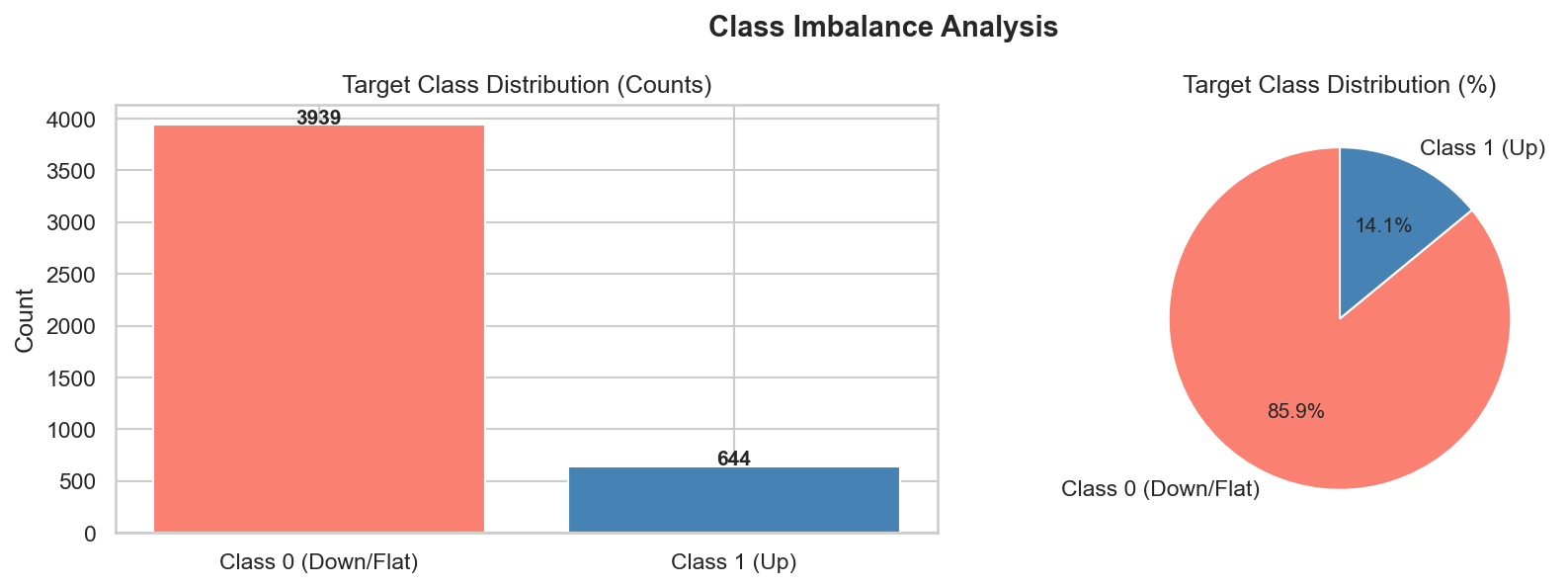
The target class is highly imbalanced — only ~13.7% of trading days produce a ≥1% SPY gain (class 1). The remaining ~86.3% are flat or negative days (class 0).
Why Imbalance Matters
A naive model that predicts “0 every day” achieves ~86% accuracy but zero utility—it never generates a buy signal. This is the accuracy paradox: a high-accuracy model can be completely useless when classes are skewed.
The imbalance directly drives three design decisions downstream:
- HPT metric: Accuracy is a misleading optimisation target. We use F1 score instead—the harmonic mean of precision and recall—which penalises models that ignore the minority class.
- Class weights: All three models use
class_weight="balanced"(Logistic Regression, Random Forest) orscale_pos_weight(XGBoost) to up-weight the minority class during training. - Calibration check: We verify in Part IV that predicted probabilities are meaningful, not just scores—because strategy thresholds depend on calibrated probabilities.
Imbalance Ratio
For the spy_run training data (SPY 2006 – Feb 2024):
- Class 0 (flat/down): ~86.3% of days
- Class 1 (≥1% up): ~13.7% of days
- Imbalance ratio: approximately 6.1:1
Feature Signal Analysis
Mutual Information
Mutual information (MI) quantifies the statistical dependence between each feature and the binary target. Unlike Pearson correlation, MI captures non-linear relationships and is invariant to monotone transforms.
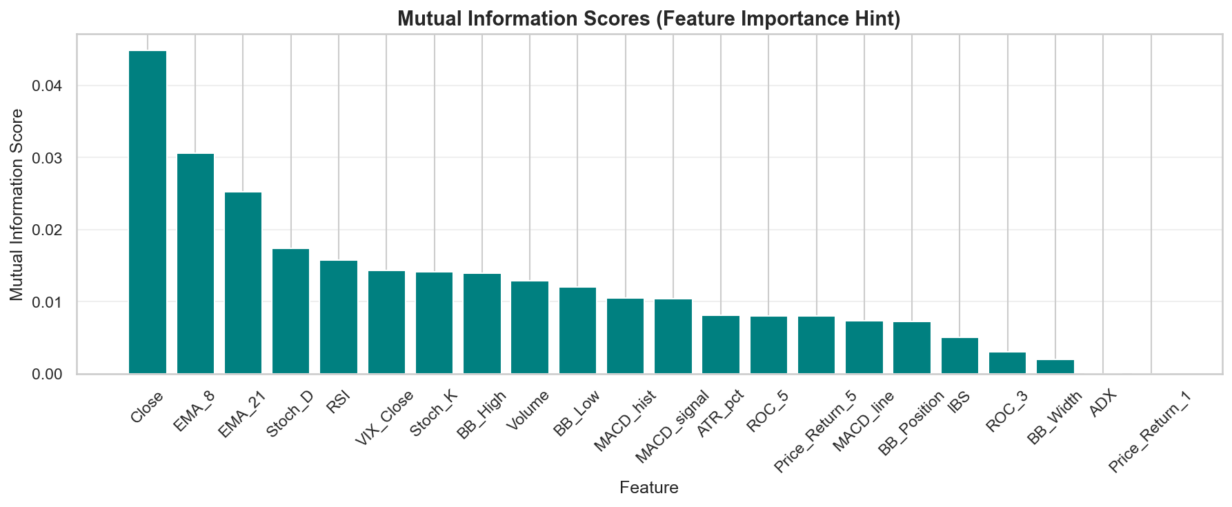
Higher MI scores indicate more predictive signal. Features with near-zero MI provide essentially no information about whether the next day will be a ≥1% up day.
The MI analysis reveals a clear ranking. Key findings:
- Close and price-level features carry the strongest MI signal—reflecting the fact that large absolute price moves (≥1%) are more common at higher price levels (higher dollar volatility).
- VIX_Close and volatility-based features have moderate-to-strong MI. High-volatility environments produce more large moves in both directions.
- Momentum oscillators (RSI, Stoch_K, ROC_3) have moderate MI—they capture mean-reversion and momentum cycles.
- Pure trend features (ADX) and short-term returns (
Price_Return_1) have the lowest MI for this specific task.
Correlation Analysis
| A Pearson correlation heatmap across all features identifies redundant pairs. Features that are strongly correlated with each other ( | r | > 0.85) add computational cost without independent information. |
Key redundancies found:
EMA_8andEMA_21are highly correlated with each other and withClose(r > 0.99)—they essentially re-encode the price level BB_Lowis nearly identical toClose(r = 0.998) MACD_lineandMACD_signalare correlated by construction (signal is a smoothed MACD line,r = 0.948) Stoch_KandStoch_Dare correlated (D is a 3-day smooth of K,r = 0.906) ROC_5andPrice_Return_5are perfectly correlated (r = 1.0) BB_Position,RSI, andStoch_Kform a correlated cluster (all measure overbought/oversold conditions)
Combined with the MI scores, this drives the feature dropping decisions below.
Feature Distributions & Skewness
Before selecting transforms, we inspect the raw distributions of all features.
Several features show heavy right-skewed distributions:
| Feature | Skewness (raw) | Issue |
|---|---|---|
BB_Width | 3.33 | Occasional volatility spikes inflate the tail |
ATR_pct | 3.17 | Same issue as BB_Width |
VIX_Close | 2.42 | Right tail from crisis periods |
Volume | 2.29 | Right tail from high-volume event days |
MACD_line, MACD_signal | -1.6 | Signed oscillators with asymmetric tails |
Skewed features create two problems:
- Logistic Regression is sensitive to outliers in the feature space—extreme values pull the decision boundary
- StandardScaler produces large Z-scores for outliers, effectively making them dominate the model
Feature Engineering Decisions
The EDA notebook writes all decisions to eda_recommendations.json:
{
  "log1p_transforms": ["ATR_pct", "BB_Width", "VIX_Close", "Volume"],
  "signed_log1p_transforms": ["MACD_line", "MACD_signal"],
  "redundant_drops": ["ATR_pct", "Close", "BB_Low", "EMA_8", "EMA_21",
                       "BB_Width", "BB_Position", "Stoch_K", "Stoch_D",
                       "MACD_signal", "Price_Return_5"]
}
The feature engineering notebook (04_feature_engineering.ipynb) reads this file and applies the transforms—keeping the two stages separate so changes to EDA recommendations automatically propagate.
Log1p Transforms
For right-skewed non-negative features, we apply log1p(x) — which maps 0→0 and compresses large values:
df["Volume"] = np.log1p(df["Volume"])
df["BB_Width"] = np.log1p(df["BB_Width"])
df["ATR_pct"] = np.log1p(df["ATR_pct"])
df["VIX_Close"] = np.log1p(df["VIX_Close"])
For signed oscillators (MACD features), we use the sign-preserving variant:
df["MACD_line"] = np.sign(x) * np.log1p(np.abs(x))
This preserves the direction of the signal while compressing extreme magnitudes.
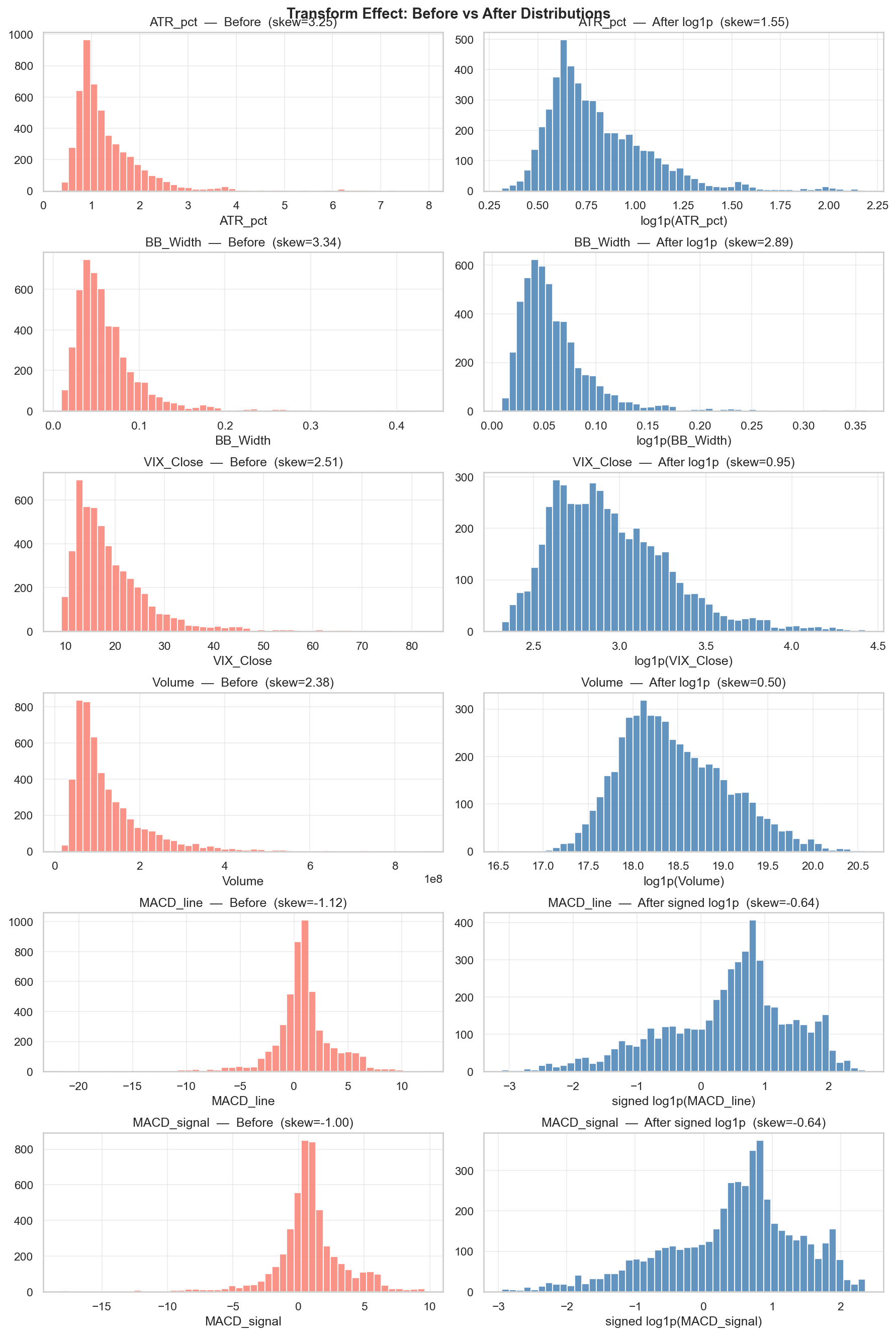
Before/after distributions for transformed features. Skewness drops significantly—Volume goes from 2.29 to 0.50, VIX_Close from 2.42 to 0.95. The MACD features become visually more symmetric around zero after the signed log1p transform. These better-behaved distributions improve Logistic Regression performance and stabilise Z-score normalization.
Feature Dropping
Features meeting either of these criteria are dropped:
High correlation with a retained feature ( r > 0.85): redundant, wastes model capacity - Near-zero MI combined with near-zero Pearson correlation: the feature contributes no detectable linear or non-linear signal
11 features are dropped, leaving a final set of 12 features:
| Category | Retained |
|---|---|
| Volume | Volume (log1p) |
| Macro | VIX_Close (log1p) |
| Volatility | BB_High |
| Trend | ADX |
| Momentum | RSI, MACD_line (signed log1p), MACD_hist, ROC_3, ROC_5, Price_Return_1, IBS |
| Price | Close |
Dropped: ATR_pct (correlated with VIX_Close), BB_Low (correlated with Close), BB_Width (correlated with ATR_pct), BB_Position (correlated with RSI/Stoch_K), EMA_8, EMA_21 (correlated with Close), MACD_signal (correlated with MACD_line), Stoch_K, Stoch_D (correlated cluster with BB_Position/RSI), Price_Return_5 (identical to ROC_5).
Temporal Split Design
The EDA and all downstream notebooks operate on training data only—the test set (last 2 years) is never touched until the final evaluation notebook. This reflects a strict no-peeking policy:
Full dataset (2006 – Feb 2026):
├── Training + Validation (2006 – Feb 2024): 4,583 rows
│   ├── Fold 1 train | Fold 1 val
│   ├── Fold 2 train | Fold 2 val
│   ├── ...
│   └── Fold 5 train | Fold 5 val
└── Test (Feb 2024 – Feb 2026): 502 rows ← never used until notebook 07
EDA, feature selection, and log1p transforms are all determined from training data—the test set’s distribution is irrelevant to these decisions.
Key Takeaways
- Class imbalance (~86/14) is the dominant challenge. Every downstream decision—HPT metric, class weights, calibration—flows from this.
- Close and VIX carry the strongest MI signal for ≥1% moves. Price level matters because higher absolute prices produce larger dollar moves, and VIX captures the volatility regime.
- Log1p transforms are necessary for Volume, BB_Width, ATR_pct, and VIX_Close—their right tails would otherwise dominate normalization and distort Logistic Regression.
- Aggressive redundancy pruning removes 11 features (from 22 to 12), eliminating correlated clusters that add noise without independent signal.
- EDA-to-engineering linkage via JSON keeps the pipeline honest: the feature engineering notebook re-reads EDA decisions rather than hard-coding them.
What’s Next?
In Part III, we establish baselines, train three ML models with hyperparameter tuning, and analyse learning curves—all with strict expanding-window cross-validation to prevent lookahead.
← Previous: Part I: Problem Statement & Technical Indicators
Next Post → Part III: Baseline Models, ML Models & Hyperparameter Tuning
References
- Mutual Information for Feature Selection - scikit-learn docs
- Imbalanced Classification Strategies - imbalanced-learn
- Log Transform for Skewed Data - Statistics How To
- F1 Score vs Accuracy - Wikipedia