Stock Return Classifier (Part III): Baseline Models, ML Models & Hyperparameter Tuning

February 17, 2026 10 minute read

This post is part of a series on building a supervised ML pipeline to classify SPY daily returns.

← Previous: Part II: EDA, Feature Selection & Feature Engineering

Next Post → Part IV: Test Evaluation & Portfolio Backtesting

⚠️ Disclaimer

This blog series is for educational and research purposes only. The content should not be considered financial advice, investment advice, or trading advice. Trading stocks and financial instruments involves substantial risk of loss and is not suitable for every investor. Past performance does not guarantee future results. Always consult with a qualified financial advisor before making investment decisions.

Introduction

In Part II, we analysed the data and engineered the features—going from 22 raw indicators down to 12 after log1p transforms and redundancy pruning. Now the modelling work begins.

Before training complex models, we need baselines—simple benchmarks that any ML model must beat to be worth deploying. Then, we train three classifiers with temporal cross-validation and grid-search hyperparameter tuning. Finally, learning curves reveal whether the models are overfitting, underfitting, or data-hungry.

Temporal Cross-Validation: The Critical Foundation

Financial time series have a property that makes standard cross-validation dangerous: temporal ordering matters. Training on future data to predict the past would produce wildly optimistic validation scores that don’t reflect real-world performance.

Expanding Window CV

We use expanding window cross-validation with 5 folds:

Data timeline: [============================================]
                2006                                  Feb 2024

Fold 1: Train [====]          | Val [==]
Fold 2: Train [======]        | Val [==]
Fold 3: Train [=========]     | Val [==]
Fold 4: Train [============]  | Val [==]
Fold 5: Train [==============]| Val [==]
                                        | Test [======] → Feb 2026

Each fold’s training set grows by one block—simulating a model that retrains on all available history. Validation always falls after training chronologically. The test set (last 2 years) is never touched during this entire stage.

Why Not Standard K-Fold?

Standard K-fold randomly shuffles data before splitting. For a time series, this means:

Training on June 2020 data while evaluating on March 2020 data
The model sees future information during training
Validation scores become unrealistically inflated

Expanding window CV avoids this by maintaining strict temporal order.

Baseline Models

Baselines serve as the minimum bar any ML model must clear. They also reveal the practical difficulty of the task—if a simple rule achieves near-ML performance, the marginal value of complex models is limited.

We evaluate two baselines on all 5 validation folds:

1. Majority-Class Classifier

Always predicts class 0 (flat/down day). Achieves ~86% accuracy but F1 = 0 because it never predicts a buy signal.

y_pred = np.zeros(len(y_val))  # always predict 0

This demonstrates the accuracy paradox: a high-accuracy model can be worthless. It also establishes why we use F1 as the optimisation metric.

2. MACD Momentum Rule

Predicts 1 (buy) when the MACD histogram is positive (short-term momentum bullish):

y_pred = (X_val["MACD_hist"] > 0).astype(int)

This is a classic momentum strategy. It achieves moderate recall (~0.39) but poor precision (~0.12)—it doesn’t discriminate well between genuine ≥1% days and ordinary positive-momentum days.

Baseline Results

Baseline model comparison

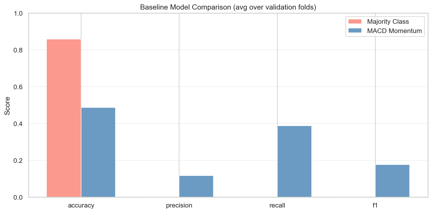
Two baselines across validation folds: (1) majority-class — ~86% accuracy, F1=0, useless as a buy signal; (2) MACD momentum rule — moderate recall but low precision (~0.12), F1≈0.18. These set the minimum bar that ML models must clear to be considered useful.

Baseline	Avg Precision	Avg Recall	Avg F1
Majority Class	0.000	0.000	0.000
MACD Momentum	~0.12	~0.39	~0.18

Any ML model that can’t beat F1 ≈ 0.18 with better precision is not adding meaningful value over a simple rule.

ML Models

Three models are trained with class_weight="balanced" (Logistic Regression, Random Forest) or scale_pos_weight (XGBoost) to handle the 6.1:1 class imbalance:

Logistic Regression

A linear classifier with L2 regularisation. Simple, fast, and interpretable—the coefficients directly show which features push the probability toward class 1.

Tuned parameter:

C (inverse regularisation strength): grid [0.01, 0.1, 1, 10, 100]

Lower C → stronger regularisation → simpler model. With 12 features and ~4,600 training rows, moderate regularisation (C around 1–10) typically works well.

Random Forest

An ensemble of decision trees where each tree is trained on a bootstrap sample with a random feature subset at each split. Inherently handles non-linear interactions between features.

Tuned parameters:

{
  "n_estimators": [50, 100, 200],
  "max_depth": [3, 5, 10, null],
  "min_samples_split": [2, 5]
}

max_depth=null allows fully grown trees (high variance, low bias). min_samples_split=5 requires at least 5 samples per leaf—a soft depth limiter that reduces overfitting.

XGBoost

Gradient boosted trees—sequential ensemble where each tree corrects the errors of the previous. Generally the strongest performer on tabular data but requires more careful tuning to avoid overfitting.

Tuned parameters:

{
  "n_estimators": [50, 100, 200],
  "max_depth": [3, 5, 7],
  "learning_rate": [0.01, 0.1, 0.3]
}

Low learning rate with more trees tends to generalise better than high learning rate with fewer trees.

Hyperparameter Tuning

Grid search over all hyperparameter combinations, averaged across all 5 validation folds, optimising F1.

Why F1 as the HPT Metric?

Accuracy is misleading at 86/14 class split
Precision alone optimises for avoiding false positives—but may produce a model that rarely fires
Recall alone optimises for catching all up days—but floods the signal with false positives
F1 (harmonic mean of precision and recall) penalises both extremes and rewards balance

For a buy signal, we want some precision (not trading on every possible signal) and some recall (not missing all the big up days). F1 reflects this balance.

HPT Implementation

from itertools import product

best_score = -np.inf
for params in product(*param_grid.values()):
    param_dict = dict(zip(param_grid.keys(), params))
    model.set_params(**param_dict)

    fold_scores = []
    for train_fold, val_fold in expanding_window_folds:
        model.fit(X_train_fold, y_train_fold)
        y_pred = model.predict(X_val_fold)
        fold_scores.append(f1_score(y_val_fold, y_pred))

    avg_score = np.mean(fold_scores)
    if avg_score > best_score:
        best_score = avg_score
        best_params = param_dict

The best hyperparameters are then used to re-fit the model on the full training set (all 5 folds combined) before saving.

Model Comparison

Model comparison

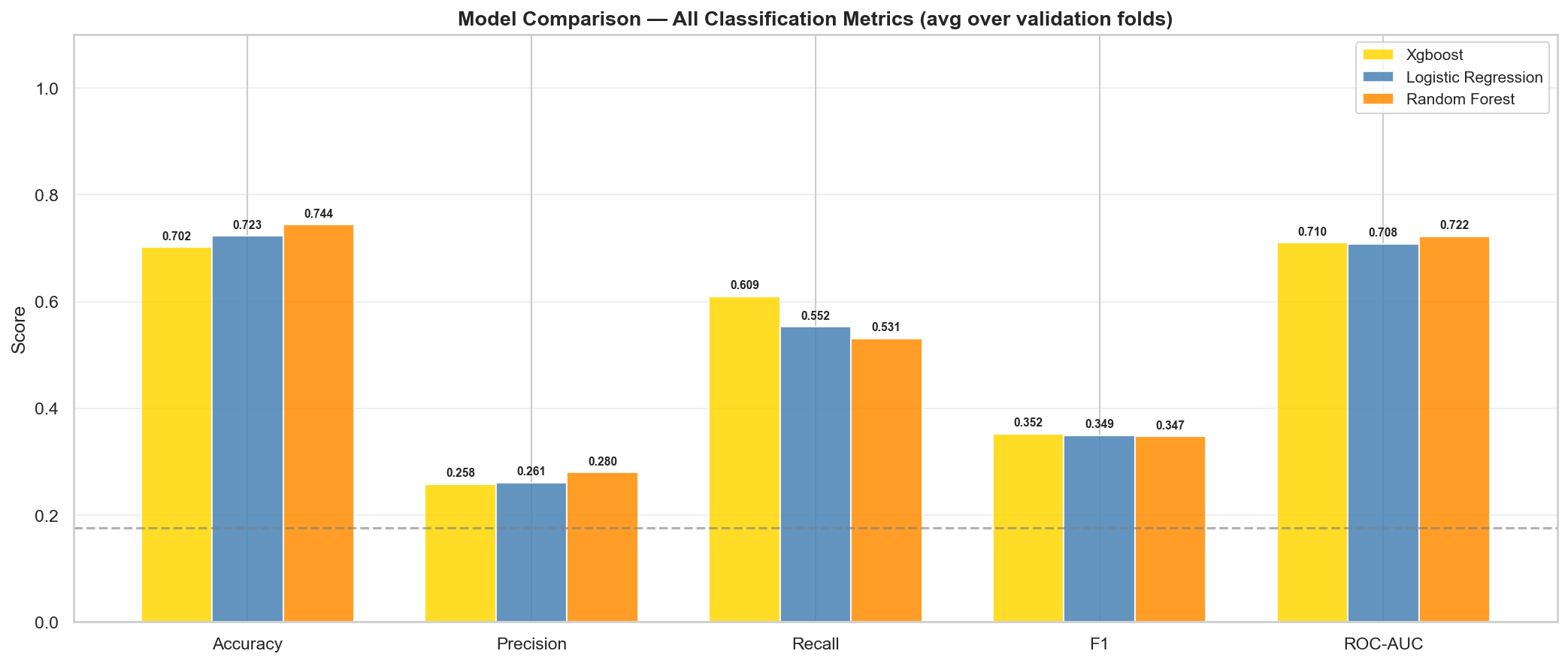
All three models evaluated on honest cross-validation (train on each fold’s training split, evaluate on its held-out validation split). All models achieve similar F1 scores within a tight band, with XGBoost slightly ahead on F1 and Random Forest leading on ROC-AUC.

Model	Avg Val Precision	Avg Val Recall	Avg Val F1	Avg Val ROC-AUC
Logistic Regression	0.261	0.553	0.349	0.708
Random Forest	0.280	0.531	0.347	0.722
XGBoost	0.258	0.609	0.353	0.710

Model Selection: F1 Tolerance + ROC-AUC Tiebreak

Rather than picking the model with the single highest F1 score, we use a two-stage selection process:

F1 dominance check: If one model leads all others by > 0.05 in F1, it is selected outright
ROC-AUC tiebreak: If multiple models fall within the 0.05 F1 tolerance band, the one with the highest ROC-AUC is selected

In this run, all three models achieve F1 scores within 0.006 of each other (0.347–0.353)—well within the ±0.05 tolerance. The selection falls to ROC-AUC, where Random Forest leads at 0.722.

Why ROC-AUC for tiebreaking? ROC-AUC measures the quality of the model’s probability ranking—how well it separates positive and negative examples across all thresholds. This directly matters for the confidence-threshold portfolio strategies (Strategy 2 and 3), where better probability ranking translates to more effective position sizing.

Learning Curves

Learning curves show how model performance evolves as training data grows—from 10% to 100% of the available training set. They answer two questions:

Is the model overfitting? (large gap between train and val scores)
Would more data help? (val score still rising at 100%)

Learning curves

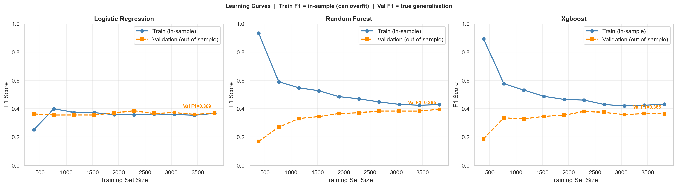
Train and validation F1 as training set size increases from 10% to 100%. The last validation fold is held out as a fixed evaluation set at all training sizes—preventing the evaluation set from shifting as the training pool grows.

No-Leakage Learning Curve Design

A subtle bug in naive learning curve implementations: if you use all 5 folds for evaluation, the validation set changes as training size grows (earlier training points borrow from folds that later become evaluation data). This inflates scores at small training sizes.

Our fix: hold out the last fold as a fixed evaluation set at all training sizes. The training pool grows from folds 1–4 progressively, while fold 5 always serves as the evaluation target.

# Fixed eval set: last fold
X_eval, y_eval = val_folds[-1]

# Training pool: all folds except last
train_pool = pd.concat([f[0] for f in val_folds[:-1]])

for size in train_sizes:
    n = int(len(train_pool) * size)
    X_sub, y_sub = train_pool.iloc[:n], y_pool.iloc[:n]
    model.fit(X_sub, y_sub)

    train_score = f1_score(y_sub, model.predict(X_sub))
    val_score = f1_score(y_eval, model.predict(X_eval))

What the Curves Show

Random Forest shows the characteristic tree-ensemble pattern: high train F1 at small sizes (memorisation) that converges downward as more samples constrain the trees. The train-val gap closes as training data grows.
Logistic Regression shows a smaller but persistent gap—lower variance but also lower capacity for the non-linear structure in the data.
Validation scores plateau around 60–70% training size for all models—suggesting the current feature set is the bottleneck, not the volume of training data.

Best Model: Random Forest

Random Forest is saved as models/{project}/best_model.pkl after re-fitting on the full training dataset (all validation folds included):

best_rf = RandomForestClassifier(
    n_estimators=100,
    max_depth=5,
    min_samples_split=2,
    class_weight="balanced",
    random_state=42,
)
best_rf.fit(X_train_full, y_train_full)

Re-fitting on the full training set (not just the last fold) ensures maximum data utilisation before test evaluation.

Key Takeaways

Expanding window CV is non-negotiable for financial time series. Standard K-fold would inflate scores and lead to overconfident model selection.
F1 is the right HPT metric at this imbalance ratio—optimising accuracy or precision alone leads to degenerate solutions.
All three models perform similarly on F1—within a 0.006 range. The ROC-AUC tiebreak selects Random Forest for its superior probability ranking (0.722 vs. 0.708–0.710).
Learning curves plateau early—additional training data contributes marginal improvement. Feature quality matters more than dataset size for this task.
Learning curve leakage is subtle: holding out a fixed evaluation fold prevents the evaluation set from shifting as training size grows.

What’s Next?

In Part IV, we evaluate the best model on the held-out 2-year test period—never-seen data—and walk through three ML portfolio strategies plus MACD and DCA baselines to quantify the economic value of the predictions.